They ob- tained rates in probability for the cumulative sum (CUSUM) change-point estimator and gave a rate of convergence of the estimator that gets worse.
arXiv:0710.4217v1 [math.ST] 23 Oct 2007
The Annals of Statistics 2007, Vol. 35, No. 4, 1802–1826 DOI: 10.1214/009053606000001596 c Institute of Mathematical Statistics, 2007
OPTIMAL RATE OF CONVERGENCE FOR NONPARAMETRIC CHANGE-POINT ESTIMATORS FOR NONSTATIONARY SEQUENCES By Samir Ben Hariz, Jonathan J. Wylie and Qiang Zhang1 Universit´e du Maine, City University of Hong Kong and City University of Hong Kong Let (Xi )i=1,...,n be a possibly nonstationary sequence such that L (Xi ) = Pn if i ≤ nθ and L (Xi ) = Qn if i > nθ, where 0 < θ < 1 is the location of the change-point to be estimated. We construct a class of estimators based on the empirical measures and a seminorm on the space of measures defined through a family of functions F. We prove the consistency of the estimator and give rates of convergence under very general conditions. In particular, the 1/n rate is achieved for a wide class of processes including long-range dependent sequences and even nonstationary ones. The approach unifies, generalizes and improves on the existing results for both parametric and nonparametric change-point estimation, applied to independent, short-range dependent and as well long-range dependent sequences.
1. Introduction. The change-point problem, in which one must detect a change in the marginal distribution of a random sequence, is important in a wide range of applications and has therefore become a classical problem in statistics. A comprehensive review of the subject can be found in [5]. In this paper we consider the general case of nonparametric estimation that must be used when no a priori information regarding the marginal distributions before and after the change-point is known. Although this problem has been widely studied for independent sequences, studying dependent sequences has importance for both theoretical reasons and numerous practical applications. In this paper we consider this challenging problem and develop a unified framework in which we can deal with sequences with quite general dependence structures. We prove that the rate of convergence of a Received December 2005; revised September 2006. Research supported by City University of Hong Kong contract 7001561. AMS 2000 subject classifications. 60F99, 62F10, 62F05, 62G20, 62G30. Key words and phrases. Long-range dependence, short-range dependence, nonstationary sequences, nonparametric change-point estimation, consistency, rates of convergence. 1
This is an electronic reprint of the original article published by the Institute of Mathematical Statistics in The Annals of Statistics, 2007, Vol. 35, No. 4, 1802–1826. This reprint differs from the original in pagination and typographic detail. 1
2
S. BEN HARIZ, J. J. WYLIE AND Q. ZHANG
broad family of nonparametric estimators is Op (n−1 ). This is a particularly surprising result because the dependence structure of the sequence plays absolutely no role in determining the rate of convergence. The rate Op (n−1 ) is clearly optimal because there are only n points in the sequence. For independent sequences there is a wide literature, and both parametric and nonparametric methods have been widely studied. The nonparametric problem was considered by Carlstein [4], who proposed an estimator, proved its consistency and determined a rate of convergence. D¨ umbgen [6] embedded the estimator proposed by Carlstein in a more general framework, improved the rate of convergence in probability and derived the limiting distributions for certain models. Ferger [7] considered the almost sure convergence for D¨ umbgen’s estimators. Yao, Huang and Davis [15] considered the case in which the location of the change-point can tend to either 0 or 1 as the sequence length tends to infinity. Ferger [8, 9] has investigated a number of features of change-point estimators including probability bounds and rates of weak and almost sure convergence. Since then several works have generalized these results to a weakly dependent or short-range dependent setting. In recent years the importance of long-memory or long-range dependent (LRD) processes has been realized in a wide range of applications, especially in the analysis of financial and telecommunication data. For the purposes of this paper we define real sequences (Xi )i=1,...,n to be short-range dependent P (SRD) if lim supn→∞ n−1 E[ ni=1 (Xi − E[Xi ])]2 < ∞ and LRD otherwise. Several works are concerned with the generalization of the results for independent sequences to a SRD setting. However, estimating change-points for LRD sequences poses a number of significant challenges and there are much fewer known results in this case. Parametric change-point estimation for LRD sequences, in which one typically has a priori knowledge about the marginal distributions, has been considered by a number of authors. Kokoszka and Leipus [12] considered the change in the mean for dependent observations for LRD sequences. They obtained rates in probability for the cumulative sum (CUSUM) change-point estimator and gave a rate of convergence of the estimator that gets worse as the strength of the dependence increases. The problem with a jump in the mean that tends to zero was considered by Horv´ ath and Kokoszka [11]. They proved the consistency of the estimator and gave the limiting distribution. For sequences that have a change in the mean, Ben Hariz and Wylie [2] showed that the rate of convergence does not get worse as the strength of the dependence increases and that the rate of convergence for independent sequences is also achieved for both SRD and LRD sequences. In the nonparametric setting Giraitis, Leipus and Surgailis [10] derived a number of results that focused mainly on hypothesis testing. However, to our knowledge, there are no results regarding rates of convergence of nonparametric change-point estimation for LRD sequences.
3
CHANGE-POINT ESTIMATION
In this paper we adopt a very general framework that allows us to consider a very general class of dependence structures. In particular, we make no assumption about stationarity in the dependence structure. This is especially important in practice because one can confidently make use of the proposed estimators on a sequence without checking for such stationarity (which is typically extremely difficult in practice). This framework represents a unified setting in which independent, SRD and LRD sequences can be treated. We prove the consistency of a D¨ umbgen-type estimator and show that the Op (n−1 ) rate of convergence for independent sequences is also achieved for both SRD and LRD sequences. In addition, we consider the case in which the difference between the distributions before and after the change-point tends to zero. 2. Main results. Let (Xi )i=1,...,n be a sequence in a measurable space E. The marginal distribution (which may depend on the sequence length n) is given by L (Xi ) =
�
Pn , Qn ,
if i ≤ nθ, if i > nθ,
where 0 < θ < 1 is the location of the change-point. This means that we assume first-order stationarity on either side of the change-point, but make no assumption about stationarity in the dependence structure of the sequence. Given the sequence (Xi )i=1,...,n , we aim to estimate the location of the change-point θ using an estimator of the general type 1 θˆn = min arg max{N (Dk )} , n 1≤k nθ, where
are random stationary sequences are real sequences and P+∞ (i) (j) (i) (j) with zero mean and finite variance. If k,l=−∞ |bk bl E(ǫ0 ǫk−l )| < ∞ for (j)
(j)
i, j = 1, 2, then (Zi ) exists almost surely and E((Zi )2 ) < ∞. Let r(k) = (i) (j) −α , for α > 0, supi,j=1,2 |E(ǫ0 ǫk )|. If we assume that supk | r(k+m) r(k) | ≤ Cm then |cov(Xi , Xi+m )| ≤ C ′ m−α . This example includes FARIMA processes
6
S. BEN HARIZ, J. J. WYLIE AND Q. ZHANG
with correlated innovations such as GARCH processes. It allows us to model long-range dependence and time-dependent conditional variance. These two features are frequently encountered in financial time series. So, Assumption 1 is satisfied when F is the set of the identity function. In Theorem 1 we develop conditions that can deal with countable families of functions and norms that are bounded by weighted moments. In Theorem 2 we consider the case of uncountable families. In this case we need to control the size of the family. This will be done by using covering numbers defined in Assumption 2. We begin by considering the case where the class of functions F is countable and the difference between the distributions before and after the changepoint may tend to zero as the sequence length, n, tends to infinity. This theorem essentially handles the case in which the norm is bounded by a sum of weighted moments and hence includes most commonly used parametric estimators. For f in F we set (2.8)
kf k ≡ sup(Pn (f 2 ) + Qn (f 2 ))1/2 = sup(EPn [f 2 ] + EQn [f 2 ])1/2 . n∈N
Theorem 1. (2.9)
n∈N
Assume that the norm N satisfies N (ν) ≤
X
d(f )|ν(f )|,
f ∈F
where F is a countable family of functions satisfying (2.6) and d(f ) are P positive constants such that f ∈F d(f )kf k < ∞. We assume that there exists a positive sequence bn such that (2.10)
P[N (Pn − Qn ) > bn ] → 1
as n → ∞.
Let ρ¯ = min(1 − ǫ, ρ) for any ǫ > 0, where ρ is given in (2.6). If −¯ ρ/2 (1 + ln(n)1γ−1+¯ρ/2=0 ) + nγ−1 ] → 0 (2.11) b−1 n [n
as n → ∞,
then we have (2.12)
θˆn − θ = Op (n−1 bn−2/¯ρ ).
We note that the largest possible value of ρ¯ is strictly less than unity and so as long as γ < 1/2 we will always have γ − 1 + ρ¯/2 6= 0, in which case we obtain a less restrictive condition than [6] on the speed at which the difference between the distributions before and after the jump tends to zero. Moreover, if the sequence is LRD (ρ < 1), then we have more freedom in the choice of γ, namely γ ≤ 1 − ρ/2. This theorem takes a simpler form when N (Pn − Qn ) is bounded away from zero. This is stated in following corollary.
CHANGE-POINT ESTIMATION
7
Corollary 1. Under Assumption 1, assume that the seminorm N satisfies (2.9) and (2.10) with bn ≥ b > 0. Then θˆn − θ = Op (n−1 ).
(2.13)
Corollary 1 includes the commonly encountered case in which the distributions Pn and Qn do not depend on the sequence length and the seminorm is nonrandom. Equation (2.10) controls the rate at which the seminorm of the difference between the two distributions decays to zero by stating that it decays more slowly than some sequence bn . In particular, if the seminorm is nonrandom, one can take bn = 2−1 N (Pn − Qn ). Equation (2.11) requires that random fluctuations arising from sums of the type (2.2), which have size O(n−ρ/2 + nγ−1 ), decay to zero faster than the sequence bn and consequently decay faster than the distance between the two distributions. This is a natural condition to be able to detect a change-point. We now turn our attention to the case when the family F contains an uncountable infinity of functions. The following theorem deals with an extremely general set of norms including all of those considered by Carlstein [4]. In this case, under the assumptions that the family has a finite covering number, we obtain the same rate of convergence as in (2.13) when Pn and Qn are independent of n. For the case in which the size of the difference between Pn and Qn tends to zero as n → ∞ we obtain a rate that depends on the covering number that will typically represent some loss on (2.12). Assumption 2. Given two functions l and u, the bracket [l, u] is the set of all functions f with l ≤ f ≤ u. Given a norm k · k on a space containing F , an ε-bracket for k · k is a bracket [l, u] with kl − uk < ε. The bracketing number N[·] (ε, F, k · k) is the minimal number of ε-brackets needed to cover F. A family F is said to satisfy Assumption 2 if (2.14)
∀ε > 0
N[·] (ε, F, k · kX ) < ∞,
where k · kX is a norm satisfying supn∈N |Pn (|f |)| + |Qn (|f |)| ≤ kf kX . We refer the reader to the monograph of van der Vaart and Wellner [14] for examples about bracketing numbers. The following theorem considers the case when the difference between the distributions before and after the change-point may tend to zero. Theorem 2. (2.15)
Assume that the seminorm satisfies N (ν) ≤ sup{|ν(f )|, f ∈ F},
8
S. BEN HARIZ, J. J. WYLIE AND Q. ZHANG
where F is a family of functions that satisfies sup{kf k, f ∈ F} < ∞ and Assumptions 1 and 2. Let ρ¯ = min(1 − ǫ, ρ) for any ǫ > 0, where ρ is given in (2.6), and εn be any positive sequence that tends to zero as n → ∞. We assume that there exists a positive sequence bn such that (2.16)
P(N (Pn − Qn ) > bn ) → 1
as n → ∞
and −¯ ρ/2 b−1 (1 + ln(n)1γ−1+¯ρ/2=0 ) + nγ−1 ] → 0. n N[·] (bn εn , F, k · kX )[n
Then we have 2/¯ ρ θˆn − θ = Op (n−1 [b−1 ). n N[·] (bn εn , F, k · kX )]
(2.17)
The following corollary considers the case in which the norm between the distributions before and after the change-point is strictly positive. Provided that the bracketing number is finite, the n−1 convergence rate is achieved for any norm within a class of functions satisfying Assumptions 1 and 2. Corollary 2. Under Assumptions 1 and 2, assume that the seminorm satisfies (2.10) with bn ≥ b > 0 and (2.15). Then (2.13) is satisfied. Remark 1. In the case bn > b > 0, Theorems 1 and 2 both give the same Op (n−1 ) rate for both ρ < 1 and ρ ≥ 1. For Theorem 1, in the case 2 2 bn → 0 with ρ ≥ 1, it is possible to obtain the rate Op (n−1 b−2 n ln (nbn )) which can represent a marginally better result. A similar result can be obtained for Theorem 2 with bn → 0 and ρ ≥ 1. These results can be obtained by modifying Lemma 1 of our proof using Theorem 3 in [13]. Remark 2. Assumption 1 can be replaced by the following more general, but less intuitive, condition: there exist constants C > 0 and ρ > 0, such that for any m (2.18)
sup
sup
f ∈F k,m,k+m≤n
E
k+m X
!2
[f (Xi ) − E(f (Xi ))]
i=k
≤ Cm2−ρ .
In this case kf k can be replaced by unity in the assertions of Theorems 1 and 2. Observe that this assumption is particularly weak and satisfied by a large class of processes and families of functions. We now present more examples of commonly used time series models and families of functions that satisfy (2.18) and Assumption 2. Example 6. We begin by considering a linear process with a family of functions that satisfies a Lipschitz condition. Let F be a family of uniformly
9
CHANGE-POINT ESTIMATION
bounded functions such that supf ∈F |f (x) − f (y)| ≤ C1 |x − y|η1 for some η1 > 0 and C1 > 0. Then according to [14] F satisfies Assumption 2 for any Lp norm. We now show that if the sequence is drawn from Example 5, then P (j) (j) (2.18) is satisfied under additional weak conditions. Let Xiv ≡ |k| nθ. Assume that (ǫk , ǫk ) are qdependent and E[Xi − Xiv ]2 ≤ C2 v −η2 .
∃η2 > 0 ∀v
(2.19)
(1)
(2)
For example, if |bk | + |bk | ≤ C|k|−β and β > 1/2, then one can readily show that (2.19) is satisfied. The sequence Xiv is 3v-dependent for v > q, Pk+m ¯ v 2 f (Xi )) ≤ Cmv, and so by using a blocking technique we have E( i=k 1/(1+η η ) ¯ 1 2 where f (X) = f (X) − E[f (X)]. Letting v = m , we obtain E
k+m X
!2
f¯(Xi )
i=k
≤ 2E
k+m X
v(m) f¯(Xi )
i=k
≤ Cm
2−η1 η2 /(1+η1 η2 )
!2
+ 2E
!2
k+m X
v(m) (f¯(Xi ) − f¯(Xi ))
i=k
.
So (2.18) is also satisfied and hence Theorem 2 applies. Example 7. In this example we consider a linear process given in Example 5 with a family composed of indicator functions, namely F = {fx (·) ≡ 1·≤x , x ∈ R}. This family is relevant to the commonly used Lp and L∞ norms (1) (2) in Example 1 for which Assumption 2 is satisfied. We assume that (ǫk , ǫk ) (2) (1) are q-dependent and |bk | + |bk | ≤ C|k|−β with β > 1/2. We begin by assuming that q = 1. Then we have E
k+m X i=k
!2
f¯x (Xi )
≤ 2E
k+m X
!2
f¯x (Xiv )
i=k
+ 2m2 sup E[f¯x (Xi ) − f¯x (Xiv )]2 , i
where f¯xP (X) = fx (X) − E[fx (X)]. Again, using the blocking technique, we k+m ¯ have E( i=k fx (Xiv ))2 ≤ Cmv. One can also show that for some η1 > 0, supx supi E[fx (Xi ) − fx (Xiv )]2 ≤ Cv −η1 . Then by choosing v ∼ m1/(1+η1 ) we Pk+m ¯ obtain E( i=k fx (Xi ))2 ≤ Cm2−η1 /(1+η1 ) . The case of q > 1 can be handled Pk+m ¯ by dividing the sum i=k fx (Xi ) into q blocks such that within each block the innovations are independent. Hence (2.18) is satisfied and Theorem 2 applies. Before presenting the proofs, we give an intuitive explanation of why the rate of convergence of the estimator does not depend on the dependence structure of the sequence. We define tk ≡ k/n. Then Dk ≡ Dn (tk ), where [nt]
Dn (t) = t1−γ (1 − t)1−γ
n X 1 1 X δX δX − nt i=1 i n(1 − t) i=[nt]+1 i
!
10
S. BEN HARIZ, J. J. WYLIE AND Q. ZHANG
and w(t) = tγ (1−t)γ . We rewrite Dn (t) as the sum of its mean and a centered random component, Bn (t), (2.20)
Dn (t) =
1 [(Pn − Qn )g(t) + Bn (t)], w(t)
where g(t) = t(1 − θn )1t≤θn + θn (1 − t)1t>θn is a piecewise linear function that takes its maximum at the point θn ≡ [nθ]/n and Bn is the empirical bridge measure given by (2.21)
Bn (t) = Wn (t) − tWn (1),
(2.22)
Wn (t) =
[nt]
1X [δX − L (Xi )]. n i=1 i
Our main results stated in Theorems 1 and 2 occur because of the cancellation of two competing effects. One of the effects is concerned with the absolute magnitude of the random noise in Dn (t). The mean component of Dn (t) is monotonically increasing for t < θn and monotonically decreasing for t > θn and therefore takes its maximum at t = θn . The estimator is chosen by maximizing N (Dn (t)), so if the noise is sufficiently small we would expect to obtain a good estimate. For independent or SRD sequences the partial sums in the centered random component of Dn (t), namely Bn (t), typically have a magnitude of order n−1/2 as n → ∞. As shown by D¨ umbgen, this gives rise to typical errors of order n−1 in the estimator. For LRD sequences the partial sums decay more slowly. This means that the stronger the dependence the larger the random component in (2.2). This effect makes the estimation more difficult. One might naively expect that this would mean that LRD sequences have a slower rate of convergence than SRD or independent sequences. However, there is another effect that is concerned with the variations in the noise in the vicinity of the change-point. Correlations in LRD sequences imply that the random noise Bn (t) becomes correlated. This means that the random noise has less rapid variation and local fluctuations become smaller. Estimation requires one to find the global maximum of N (Dn (t)) and this depends critically on the local variations in the vicinity of the change-point rather than on the absolute magnitude of the noise. Hence the smaller the local fluctuations are, the easier the estimation becomes. These two effects exactly compensate and give the surprising feature that the overall rate of convergence is the same for all dependence structures. 3. Simulations. In this section we present the results of numerical simulations that investigate some of the important practical features of changepoint estimation. We confirm that the rate of convergence is Op (n−1 ) for LRD, SRD and independent sequences. We also determine how large the sequence length needs to be before the Op (n−1 ) rate is observed.
CHANGE-POINT ESTIMATION
11
We considered the estimation of the change-point for a sequence that is a function of a dependent Gaussian variable, (Yi )i=1,...,n with zero mean and unit variance. We generated a sequence with a change in the marginal distribution by taking Xi =
�
Yi2 − 1, 1 − Yi2 ,
if i ≤ nθ, if i > nθ.
(a)
(b) Fig. 1. The MAE of n(θˆn − θ) for different values of α: under (a) the L1 norm and (b) the KS norm.
12
S. BEN HARIZ, J. J. WYLIE AND Q. ZHANG
The sequence (Xi ) has the property that the marginal distributions before and after the jump have the same mean and variance, but have different skewness. We generated the Gaussian sequences (Yi ) with a covariance given by r(n) = (1 + n2 )(−α/4) ∼ n−α/2 using the Durbin–Levinson algorithm (see, e.g., [3]). The sequence (Xi ) satisfies Assumption 1 with ρ = α. We note that the Durbin–Levinson algorithm has complexity O(n2 ) and so generating long sequences can be quite computationally expensive. We show results for the estimator that uses the Kolmogorov–Smirnov norm (KS) (2.4) and the L1 norm defined in (2.5) with p = 1. The parameter γ is equal to 0.5. We note, however, that taking different norms, such as p = 2 in equation (2.5), yields qualitatively similar results. We considered independent sequences, SRD sequences with α = 1.5 and LRD sequences with values of α = 1.0, 0.8, 0.6 and 0.4. We present simulations in which the sequence length, n, varies between 1000 and 7000. The mean absolute error MAE ≡ E(|(θˆn − θ)|) for each value of α was estimated using 10,000 different sequences. In Figure 1 we plot n(MAE ) against n with 95% confidence intervals. Since θˆn − θ = Op (n−1 ), we anticipate that n(MAE ) should tend to a constant as n tends to infinity. This is clearly seen in Figure 1 for independent, SRD and LRD sequences. As the range of dependence becomes longer, the value of n required to obtain the Op (n−1 ) scaling becomes larger. This is because the leading order correction to the Op (n−1 ) rate contains partial sums that are a factor n−α/2 smaller than the leading term. So for small α, large values of n are required for the leading order term to dominate the corrections. 4. Proofs. We will begin by proving that the estimators are consistent. For Theorem 1 this is straightforward, but for Theorem 2 we require a projection argument to deal with the uncountable size of the family F . Having proved consistency, we then turn our attention to the rates proofs. The rates proofs follow a similar pattern to the consistency proof and the techniques used are similar. In the proofs, C, C1 , C2 , . . . denote generic constants that are independent of n for n large enough whose values may differ in different equations. In general, θ ∈ / {k/n : k = 1, . . . , n} so we have defined θn ≡ [nθ]/n. To prove Proposition 1 below and Theorems 1 and 2 it suffices to prove the assertions with θ replaced by θn . In all of the proofs, we will assume ρ < 1 since the proofs can be easily adapted for the case ρ ≥ 1 by replacing ρ with ρ¯. We require the following lemmas for the proofs. The first one is a maximal inequality which is a special case of Theorem 1 in [13].
13
CHANGE-POINT ESTIMATION
Assume (2.6) with ρ < 1. Then there exists a constant D(ρ) >
Lemma 1. 0 such that
!2 k X E max [f (Xi ) − E(f (Xi ))] ≤ D 2 (ρ)kf k2 n2−ρ . 1≤k≤n
(4.1)
i=1
The second lemma controls the size of the empirical bridge and is a simple consequence of (4.1). Lemma 2. Assume (2.6) holds with 0 < ρ < 1. Then there exists a constant D(ρ) > 0 such that for any 0 < κ ≤ 1 (4.2)
E
�
�
sup |(Wn (t) − Wn (θn ))(f )| ≤ D(ρ)kf kn−ρ/2 κ1−ρ/2
|t−θn |≤κ
and (4.3)
�
�
E sup |(Wn (t))(f )| + sup |(Bn (t))(f )| ≤ D(ρ)kf k(n−ρ/2 κ1−ρ/2 ). |t|≤κ
|t|≤κ
The third lemma controls the size of oscillations of the weighted empirical bridge which we define as Bnw (t) ≡ w−1 (t)Bn (t). Lemma 3. Assume (2.6) with ρ < 1. Then there exist constants C(θ, η) and D(ρ) such that for κ < η, (4.4) E
�
�
sup |(Bnw (t) − Bnw (θn ))(f )| ≤ C(θ, η)D(ρ)kf kn−ρ/2 κ1−ρ/2 .
|t−θn |≤κ
Proof. Using Taylor’s theorem to expand w−1 (t) near t = θn , we obtain Bnw (t) − Bnw (θn ) = w−1 (θn )(Wn (t) − Wn (θn )) − (t − θn )[w−1 (θn )Wn (1) + (w−2 (ξ)w′ (ξ))(Wn (t) − tWn (1))], where ξ ∈ (t, θn ). Therefore, for η small enough and |t − θn | ≤ η, there exists a constant C(θ, η) such that (4.5)
|(Bnw (t) − Bnw (θn ))(f )| ≤ w−1 (θn )|(Wn (t) − Wn (θn ))(f )| + C(θ, η)|t − θn | sup |Wn (t)(f )|. 0≤t≤1
14
S. BEN HARIZ, J. J. WYLIE AND Q. ZHANG
Hence it suffices to control the size of the oscillations of Wn (t). By (4.2) and (4.3) of Lemma 2, we have E
�
sup |(Bnw (t) − Bnw (θn ))(f )| |t−θn |≤κ ≤w
−1
(θn )E
�
� �
sup |(Wn (t) − Wn (θn ))(f )|
|t−θn |≤κ
+ C(θ, η)κE
�
�
sup |Wn (t)(f )|
0≤t≤1
≤ w−1 (θn )D(ρ)kf kn−ρ/2 κ1−ρ/2 + D(ρ)kf kC(θ, η)κn−ρ/2 ≤ C(θ, η)D(ρ)kf kn−ρ/2 κ1−ρ/2 , where C(θ, η) may change in each occurrence, and the relation (4.4) follows. � 4.1. Consistency proofs. We first recall some notation and introduce some additionally. Let δn = Pn − Qn , h(t) = w−1 (t)(t(1 − θn )1t≤θn + θn (1 − t)1t>θn ) and Bnw (t) = w−1 (t)Bn (t), where Bn (t) is defined in (2.21) and w(t) = tγ (1 − t)γ . For t in Gn ≡ {k/n, 1 ≤ k < n} we rewrite Dn (t) defined in (2.20) as Dn (t) = Bnw (t) + h(t)δn . We also recall that θˆn is a maximum of {N (Dn (t)), t ∈ Gn }. The following proposition states the consistency of the estimators. Proposition 1. Let X be a sequence and F a family such that (2.6) is satisfied. Assume that the conditions of Theorem 1 or Theorem 2 are satisfied. Then ∀η > 0 P(|θˆn − θn | > η) → 0 as n → ∞. Proof of Theorem 1. By definition θˆn is a maximum of N (Dn (t)). So N (Dn (θˆn )) ≥ N (Dn (θn )).
(4.6) Using (2.20), we obtain
N (Bnw (θˆn ) + δn h(θˆn )) ≥ N (Bnw (θn ) + δn h(θn )). Repeated use of the triangle inequality yields N (B w (θˆn )) ≥ N (B w (θn ) + δn h(θn )) − N (δn h(θˆn )) n
n
≥ N (δn h(θn )) − N (δn h(θˆn )) − N (Bnw (θn )).
15
CHANGE-POINT ESTIMATION
Hence, (4.7)
N (Bnw (θˆn )) + N (Bnw (θn )) ≥ N (δn )(h(θn ) − h(θˆn )).
We define an = inf |t−θn |>η {h(θn ) − h(t)}. Then an > a > 0 for n large enough, because h is monotonically increasing for t < θn and monotonically decreasing for t > θn . Since an is defined to be an infimum we obtain P[|θˆn − θn | > η] (4.8)
= P[N (Bnw (θˆn )) + N (Bnw (θn )) ≥ aN (δn ), |θˆn − θn | > η] ≤ P[N (Bnw (θˆn )) + N (Bnw (θn )) ≥ abn , |θˆn − θn | > η] + P[N (δn ) ≤ bn ].
We use the fact that P[X + Y ≥ ε, B] ≤ P[|X| ≥ ε/2, B] + P[|Y | ≥ ε/2, B], for any random variables X and Y , set B and ε > 0, to obtain abn ˆ , |θn − θn | > η 2 � � abn w + P N (Bn (θn )) ≥ + P[N (δn ) ≤ bn ] 2 ≡ A1 + A2 + A3 . �
�
P[|θˆn − θn | > η] ≤ P N (Bnw (θˆn )) ≥ (4.9)
We begin by controlling A1 . We will assume that η is sufficiently small such that θn − η > 0 and 1 − θn − η > 0, since other cases can be dealt with similarly. For the sake of brevity we introduce the notation βmin = min(θn − η, 1 − θn − η) and βmax = max(θn − η, 1 − θn − η). We introduce sets S1 , . . . , SJ given by Sj = {t : 2−j ≤ t(θn −η)−1 < 2−j+1 } ∪ {t : 2−j ≤ (1−t)(1−θn −η)−1 < 2−j+1 }. The integer J is chosen so that n−1 2J−1 ≤ βmax < n−1 2J . As j increases these sets become increasingly close to the end points of the domain and J is chosen to be large enough so that the smallest and largest possible values of the change point (i.e., θˆn = 1/n and θˆn = 1 − 1/n) are included in one of the sets. Then (4.10)
A1 =
J X abn A˜1 (n, j), ≡ P θˆn ∈ Sj , N (Bnw (θˆn )) ≥ 2 j=1 j=1
� J X
�
where (4.11)
abn A˜1 (n, j) ≤ P sup N (Bn (t)) ≥ inf w(t) . 2 t∈Sj t∈Sj �
�
16
S. BEN HARIZ, J. J. WYLIE AND Q. ZHANG
A simple calculation shows that inf t∈Sj w(t) = min(w((θn − η)2−j ), γ w((1 − θn − η)2−j ) > βmin 2−jγ−1 . Hence applying the Markov inequality to (4.11) we obtain �
�
−γ jγ+2 −1 −1 A˜1 (n, j) ≤ βmin 2 a bn E sup N (Bn (t)) . t∈Sj
In order to control E[supt∈Sj N (Bn (t))] we need to control E[supt∈Sj |Bn (t)(f )|] for f ∈ F . We use (2.9) to prove Proposition 1 under the conditions of Theorem 1 and use a chaining argument for Proposition 1 under the conditions of Theorem 2. The control of E[supt∈Sj |Bn (t)(f )|] is formulated in Lemma 2. Using (2.9) and applying Lemma 2, we obtain �
−γ jγ+2 −1 −1 A˜1 (n, j) ≤ βmin 2 a bn E sup
X
t∈Sj f ∈F
−γ jγ+3 −1 −1 ≤ βmin 2 a bn
X
�
d(f )|Bn (t)(f )|
d(f )D(ρ)kf kn−ρ/2 (βmax 2−j )1−ρ/2 .
f ∈F
Substituting the above inequality into (4.10), we obtain −γ 1−ρ/2 −1 −1 (4.12) A1 ≤ 8βmin βmax a bn D(ρ)n−ρ/2
X
J X
d(f )kf k
2(γ−1+ρ/2)j .
j=1
f ∈F
It is easy to show that
(4.13)
J X
2(γ−1+ρ/2)j
j=1
≤ C(ρ, γ)(1 + nγ−1+ρ/2 1γ−1+ρ/26=0 + ln n1γ−1+ρ/2=0 ).
Substituting (4.13) into (4.12) and relabeling the constant yields −ρ/2 (1 + ln n1γ−1+ρ/2=0 ) + nγ−1 ) (4.14) A1 ≤ C1 b−1 n (n
X
d(f )kf k.
f ∈F
To control A2 we make similar use of the Lemma 2 to obtain −ρ/2 A2 ≤ C2 D(ρ)b−1 n n
(4.15)
X
d(f )kf k.
f ∈F
Finally from (4.9), (4.14) and (4.15) we deduce P[|θˆn − θn | > η] ≤ Cb−1 n
X
d(f )D(ρ)kf k(nγ−1 (1 + ln n1γ−1+ρ/2=0 ) + n−ρ/2 )
f ∈F
+ P(N (δn ) ≤ bn ).
17
CHANGE-POINT ESTIMATION
Taking thePlimit n → ∞ under the conditions (2.10) and (2.11) and the condition f ∈F d(f )kf k < ∞ completes the proof. �
Proof of Theorem 2. The consistency proof under the assumptions of Theorem 2 is identical to that of Theorem 1 up until (4.9). Then we proceed by using a projection argument to bound A1 , A2 , and A3 . This projection argument is to deal with the uncountable family of functions. Since N (K) ≡ N[·] (2−K , F, k · kX ) is finite for any integer K, there exists a finite sequence of pairs of functions (fiK , ∆K i )1≤i≤N (K) , such that ∀f ∈ F there exists i such K K −K . For each K we define a map M that |f − fi | ≤ ∆i , and k∆K i kX ≤ 2 K from F to F × F by M(f ) = (fi(f ) , ∆K i(f ) ) ≡ (πK (f ), ∆K (f )), where i(f ) = K K K inf{1 ≤ i ≤ N (K)|fi − ∆i ≤ f ≤ fi + ∆K i }. We assume that γ − 1 + ρ/2 6= 0 (the case γ − 1 + ρ/2 = 0 can be handled similarly and is hence omitted). We apply the Markov inequality to A1 in equation (4.9) and then use the assumption (2.15) on the seminorm N to obtain �
�
w ˆ A1 ≤ 2a−1 b−1 n E sup |Bn (θn )(f )|1|θˆn −θn |>η . f ∈F
To control A1 we will consider two cases: θˆn > θn and θˆn < θn , hence A1 ≤
2a−1 b−1 n +E
� �
E
sup |Bnw (θˆn )(f )|10