Abstract. The problem of optimal policy formulation for teams of resource-limited agents in stochastic environments is com- posed of two strongly-coupled ...
Optimal Resource Allocation and Policy Formulation in Loosely-Coupled Markov Decision Processes Dmitri A. Dolgov and Edmund H. Durfee Department of Electrical Engineering and Computer Science University of Michigan Ann Arbor, MI 48109 {ddolgov, durfee}@umich.edu Abstract The problem of optimal policy formulation for teams of resource-limited agents in stochastic environments is composed of two strongly-coupled subproblems: a resource allocation problem and a policy optimization problem. We show how to combine the two problems into a single constrained optimization problem that yields optimal resource allocations and policies that are optimal under these allocations. We model the system as a multiagent Markov decision process (MDP), with social welfare of the group as the optimization criterion. The straightforward approach of modeling both the resource allocation and the actual operation of the agents as a multiagent MDP on the joint state and action spaces of all agents is not feasible, because of the exponential increase in the size of the state space. As an alternative, we describe a technique that exploits problem structure by recognizing that agents are only loosely-coupled via the shared resource constraints. This allows us to formulate a constrained policy optimization problem that yields optimal policies among the class of realizable ones given the shared resource limitations. Although our complexity analysis shows the constrained optimization problem to be NP-complete, our results demonstrate that, by exploiting problem structure and via a reduction to a mixed integer program, we are able to solve problems orders of magnitude larger than what is possible using a traditional multiagent MDP formulation.
Introduction We address the problem of finding optimal policies for teams of resource-limited autonomous agents that operate in stochastic environments. While various aspects of this problem have received significant amounts of attention, there has been limited focus on addressing the combined problem of deciding how the limited shared resources should be distributed between the agents and what policies they should adopt, such that the social welfare of the team is maximized. Notice that in this problem formulation, figuring out the value of a particular allocation requires one to solve a stochastic policy optimization problem. Hence, the resource allocation and the policy optimization problems are very closely coupled. A straightforward approach to solving this problem is to formulate both the resource allocation process and the c 2004, American Association for Artificial IntelliCopyright gence (www.aaai.org). All rights reserved.
actual operation of the agents as a large multiagent MDP (Boutilier 1999) on the joint state and action spaces of all agents. However, this method suffers from an exponential increase in the size of the state space, and thus very quickly becomes infeasible for teams of reasonable size. A common way of addressing this problem of large state spaces in MDPs is based on problem decomposition (Boutilier, Brafman, & Geib 1997; Dean & Lin 1995; Meuleau et al. 1998; Singh & Cohn 1998), where a global MDP is decomposed into several independent or looselycoupled sub-MDPs. These sub-MDPs are usually solved independently and the resulting policies are then combined to yield a (perhaps suboptimal) solution to the original global MDP. In this work, we focus on domains where the agents operate mostly independently, but their policy optimization problems are coupled via the resources that they share. Such loose coupling of the agents makes these problems very well suited for the decomposition solution methods mentioned above. However, the existing methods either do not allow one to completely avoid the explicit enumeration of the joint states and actions (Singh & Cohn 1998) or provide only approximate solutions (Meuleau et al. 1998) to the global policy optimization problems. We present a method that does not sacrifice optimality and, by fully exploiting the structure of the problem, makes it possible to solve problems orders of magnitude larger than what is possible using traditional multiagent MDP techniques. Unlike the standard decomposition techniques, we do not divide the problem into subproblems and then recombine the solutions. Instead, we formulate one policy optimization problem with constraints that ensure that the policies do not over-consume the shared resources. The main contributions of this work are that we formally analyze the complexity of this constrained optimization problem and give a reduction of the problem to a mixed integer linear program (MILP), which allows us to capitalize on efficient methods of solving MILPs. We begin by giving a very broad, high-level description of the problem and presenting a simple example of a domain where such problems arise. We then present a formal description of our model and the problem formulation as well as an analysis of the complexity of this optimization problem and the structure of the solutions. The last sections of
General Problem Description
(a)
(b)
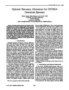
Figure 1: A resource allocation and stochastic planning problem. Once the shared operationalization resources are distributed among the agents (a), they proceed to execute the best realizable policies (b).
the paper describe our method for solving this problem and present some empirical results.
Motivating Example Imagine a group of agents that are operating autonomously – for example, a group of rovers performing a scientific mission on a remote planet. There is a clear need for coordination and task allocation among the agents in order for them to perform their mission efficiently. For instance, if the mission involves taking measurements of the soil in one location and doing a video survey of another area, it might be beneficial to assign one rover to do soil sampling, and another to do the video survey. However, the agents typically need different equipment to carry out different tasks, and while it is sometimes feasible to design and build an agent for a certain task, often if is more effective to create a generalpurpose agent that can be outfitted with different equipment depending on the task at hand. In particular, in our rover example, there might be a base station that is used as a centralized location to store consumable execution resources (fuel, energy, etc), as well as equipment (video cameras, extra batteries, etc.) that can be used to outfit the rovers for various tasks. It is certainly natural to assume that these resources are limited. Thus, a problem of efficient allocation of the shared resources arises. However, the resource allocation problem is complicated by the fact that it is often hard to calculate the exact utility of a particular assignment of the resources. Indeed, agents operating in complex environments are not able to perfectly and deterministically reason about the effects of their actions, and therefore it is necessary to adopt a model that allows one to express the uncertainty of the agents’ interactions with the environment. In fact, an agent that adopts a deterministic model of the environment and does not have contingency plans might find itself acting rather poorly. For instance, it has been estimated that the 1997 Mars Pathfinder, which did not take the uncertainty of the environment into account, spent between 40% to 75% of its time doing nothing due to plan failures (Bresina et al. 2002). Therefore, in order to determine the value of a particular resource allocation for agents operating under uncertainty, it is necessary to solve a stochastic optimization problem.
More generally, it is often the case that an agent has many capabilities that are all in principle available to it, but not all combinations are realizable within the architectural limitations, because choosing to enable some of the capabilities might usurp resources needed to enable others. In other words, a particular policy might not be operational because the agent’s architecture does not support the combination of capabilities required for that policy. If this is the case, we say that the agent exhibits operationalization constraints. At a high level, we model the situation described above as follows (illustrated in Figure 1). The agents have a set of actions that are potentially executable, but each action requires a certain combination of resources. The amount of these shared resources is limited. Furthermore, each agent has constraints as to what resources it can make use of (for example, what equipment it can be outfitted with). In our model, execution begins with a distribution of the shared resources among the agents (Figure 1a). Any resulting resource allocation must obey the constraints that no shared resource is over-utilized, i.e., the amount of all resources that are assigned to the agents does not exceed the total available amount. Furthermore, the assignment must satisfy the local constraints of the agents as to the resources that they can use. For example, it is useless (and thus essentially invalid) to assign to an agent more equipment than it can carry. Once the shared resources are distributed among the agents, they should use these resources to carry out their policies (Figure 1b) in such a way that the social welfare of the group (sum of individual rewards) is maximized.
The Model Before we describe our world model in more detail, let us note that although it is very easy to adapt our model and solution algorithms to a scenario that involves consumable execution resources (e.g., fuel, time) in addition to discrete operationalization resources (e.g., equipment to outfit the agents), we do not model the former in this paper for the ease of exposition. It turns out that including such continuous consumable resources in the model does not add to the complexity of the problem, but introduces some subtleties to the optimization and has an effect on the structure of the optimal policies (Dolgov & Durfee 2003). We briefly describe how such constraints can be incorporated into our model at the end of the subsequent section that presents our solution method. The stochastic properties of the environments in the problems that we address in this work lead us to adopt the Markov model as the underlying formalism. In particular, we use the stationary, discrete-time Markov model with finite state and action spaces (Puterman 1994). The choice is due to the fact that MDPs provide a well-studied and simple, yet a very expressive, model of the world. This section briefly describes standard unconstrained Markov decision processes and discusses the assumptions that are specific to the problems that we focus on in this work.
Markov Decision Processes A classical unconstrained single-agent MDP can be defined as a tuple hS, A, P, Ri, where: • S = {i} is a finite set of states. • A = {a} is a finite set of actions. • P = [piaj ] : S × A × S → [0, 1] defines the transition function. The probability that the agent goes to state j if it executes action a in state i is piaj . • R = [ria ] : S × A → < defines the rewards. The agent gets a reward of ria for executing action a in state i. A policy is defined as a procedure for selecting an action in each state. A policy is said to be stationary if it does not depend on time, but only on the current state, i.e., the same procedure for selecting an action is performed every time the agent encounters a particular state. A deterministic policy always chooses the same action for a state, as opposed to a randomized policy, which chooses actions according to some probability distribution over the set of actions. The term pure is used to refer to stationary deterministic policies. A randomized Markov policy π, can be described as a mapping of states to probability distributions over actions, or equivalently, as a mapping of state-action pairs to probability values: π = [πia ] : S × A → [0, 1]; πia defines the probability of executing action a, given that the agent is in state i. We assume that an agent must execute an action (a P noop is considered a trivial action) in every state, thus a πia = 1. A pure policy can be viewed as a degenerate case of a randomized policy, for which there is only one action for each state that has a nonzero probability of being executed (that probability is obviously 1). Clearly, the total probability of transitioning out of a state,Pgiven a particular action, cannot be greater than 1, i.e., j piaj ≤ 1. As discussed below, often we are actually P interested in domains where there exist states for which j piaj < 1. If, at time 0, the agent has an initial probability distribution α = [αi ] over the state space, and the system obeys the Markov assumption (namely that the transition probabilities depend only on the current state and the chosen action), the system’s trajectory (defined as a sequence of probability distributions on states) will be as follows: e t, ρt+1 = Pρ
ρ0 = α,
(1)
where ρt = [ρti ] is the probability distribution of the system at time t (ρti is the probability of being in state i at time t), e = [e and P pij ] is the Ptransition probability matrix implied by the policy (e pij = a piaj πia ).
Assumptions Typically, Markov decision problems are divided into two categories: finite-horizon problems, where the total number of steps that the agent spends in the system is finite and is known a priori, and infinite-horizon problems, where the agent is assumed to stay in the system forever (see, for example, (Puterman 1994)).
In this work we focus on dynamic real-time domains, where agents have tasks to accomplish. This leads us to make a slightly different (although, certainly, not novel) assumption about how much time the agent spends executing its policy. We assume that there is no predefined number of steps that the agent spends in the system, but that optimal policies always yield transient Markov processes (Kallenberg 1983). A policy is said to yield a transient Markov process if the agent executing that policy will eventually leave the corresponding Markov chain, after spending a finite number of time steps in it. Given a finite state space, this assumption implies that the Markov chain corresponding to the optimal policy has no recurrent states (states that have a nonzero probability of being visited infinitely many times) or, in other words: limt→∞ ρi (t) = 0. This means that there has to be some “leakage” of probability out of the system, there have to exist some states {i} for which P P i.e., a p < 1. j a ij We also assume that the rewards that an agent receives while executing a policy are bounded. Given these assumptions about bounded rewards and the transient nature of our problems, the most natural policy evaluation function to adopt is the expected total reward: V (π, α) =
T X X t=0
i
ρti
X
πia ria ,
(2)
a
where T is the number of steps during which the agent accumulates utility. For a transient system with bounded rewards, the above sum converges for any T . If the system obeys the Markov assumption and, as a result, follows the trajectory in (eq. 1), the value of a policy can be expressed in terms of the initial probability distribution, transition probabilities, and rewards as follows: ∞ ∞ X X e t α, Rρ(t) = RP (3) V (π, α) = t
t
which, under our assumptions, becomes: e −1 α V (π, α) = R(I − P)
(4)
It is clear that the value of a policy depends on the initial state probability distribution α. Moreover, in general, the relative order of two policies can change depending on the initial probability distributions, i.e., ∃π, π 0 , α, α0 : V (π, α) > V (π 0 , α), and V (π, α0 ) < V (π 0 , α0 ). However, often, there exist policies that are optimal for any initial probability distribution, i.e., V (π ∗ , α) ≥ V (π, α) ∀π, α. These policies are the ones that are commonly called “optimal” in the unconstrained MDP literature and are typically computed via dynamic programming, based on Bellman optimality equations (Bellman 1957). We refer to these policies as uniformly optimal (using the terminology from (Altman 1999)). These uniformly optimal policies π ∗ always produce a history of states that is at least as good as a history produced by any other policy, regardless of the initial conditions. Therefore, if uniformly optimal policies exist, it is sufficient to compute a single uniformly optimal policy and use it for all instances of the problem with arbitrary initial probability distributions.
However, as it turns out, uniformly optimal policies do not always exist for constrained problems that involve limited resources (we will prove this statement below). We are, therefore, interested in finding optimal policies for a given initial probability distribution α. Let us note that, although in this work we focus on transient systems with the total expected reward optimization criterion, our model, the complexity results, and the solution algorithm can be easily adapted to other commonlyused Markov models (finite horizon, infinite horizon with discounted or per-unit rewards).
Problem Description Multi-Agent Markov Decision Processes Let us now consider a multiagent environment with a set of n agents M = {m} (|M| = n), each of whom has its own set of states Sm = {im } and actions Am = {am }. Without any loss of generality, we can assume that the state and action spaces are equal (Sm = Sm0 , Am = Am0 ∀m, m0 ∈ M). In general, for a multiagent MDP, we have to define a new state space that is the cross-product of the state spaces of all agents: S(M) = S n , and a new action space that is the cross-product of the actions spaces of all agents: A(M) = An . The transition and reward functions are defined on the new state and action space, i.e., P(M) : S n × An × S n → [0, 1], and R(M) : S n × An → 0 The first constraint in (eq. 5) means that the total amounts of resources that are needed by all agents do P notmexceed the total amounts that are available. Indeed, i πia is greater than zero only if agent P mmplans P to use action a with nonzero probability. Thus, a cak i πia is greater than zero when the agent plans to use actions that require resource k, in which case �X � X m θ = 1, cm πia ak a
i
and the first summation over all agents m gives the total requirements for resource k, which should not exceed cˆk . The second constraint is analogous to the first one and has the meaning that the cost of type l of the resources assigned to agent m does not exceed its cost bounds qˆlm .
a2: p=0.75, r=1, a1: p=0.75, r=1, a2: p=0.8, r=-1, c=[0,1] c=[1,0] c=[0,1] a1: p=0.25, r=1, a2: p=0.25, r=1, c=[1,0] c=[0,1] s1
s3 a2: p=1, r=0, c=[0,1]
s2 a1: p=1, r=0, c=[1,0]
a1: p=0.8, r=-1, c=[1,0]
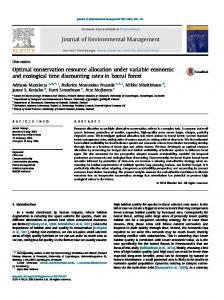
Figure 2: Uniformly-optimal policies do not always exist for constrained problems. Transition probabilities, rewards, and action costs are shown on the diagram.
Problem Properties Policy Structure In this section we show some properties of the optimal policies. We begin by demonstrating that uniformly-optimal policies (optimal for any initial distribution) do not always exist for constrained problems. This result is well known for classical constrained MDPs (Altman 1999; Puterman 1994) where constraints are imposed on the total expected costs that are proportional to the expected number of times the corresponding actions are executed. We now establish this result for problems with operationalization constraints (eq. 5) for which the costs are incurred by the agents when they include an action in their policy, regardless of how many times the action is actually executed (the costs are interpreted as the amounts of the shared resources that are required to enable the action). Proposition 1 There do not always exist uniformly-optimal solutions to problem (eq. 5). Proof: We show the correctness of the above statement by presenting an example (Figure 2) for which no uniformlyoptimal policy exists. Let us consider a problem with two identical agents (m = {1, 2}), three states {s1 , s2 , s3 }, two actions {a1 , a2 }, and two shared resource types (k = {1, 2}). The rewards (r), transition probabilities (p), and action costs (c) for all actions are shown in Figure 2. The resource costs (requirements) for action a1 are [1, 0], i.e., it needs the first resource and does not use the second one. Action a2 is exactly the opposite. States s1 and s2 are “good”, because the agents can receive positive rewards (r = 1) there, and state s3 is “bad”, since the reward there is negative (r = −1). The obvious unconstrained optimal policy for both agents is to execute action a1 in state s1 , action a2 in state s2 and either action (or a probabilistic mixture of the two) in state s3 . However, in order for both agents to be able to execute this policy, they each need to have one unit of each of the resource types. Let us now assume that there is only one unit of each resource available (ˆ c = [1, 1]), and let us show that there does not exist a policy that is optimal for all initial probability distributions α. Consider the situation where the first agent starts in state s1 and the second agent starts in state s2 , i.e., α1 = [1, 0], α2 = [0, 1]. Then, the obvious unique optimal
joint policy that satisfies the resource constraints is π 1 = [(1, 0), (1, 0), (1, 0)] and π 2 = [(0, 1), (0, 1), (0, 1)].1 The resource cost of this joint policy is [1, 1], which satisfies the constraints on the total use of the shared resources. The value (total expected reward) of that policy is zero (V (α, π) = 0), since each agent, on average, receives the positive reward (+1) five times before it transitions to state s3 , where its expected payoff is -5, yielding a total expected value of zero. This policy is clearly the unique optimum for the given initial conditions, because any other policy would either not satisfy the constraints or yield a lower (negative) payoff. If we consider a problem with the reversed initial conditions α0 where the first agent starts in state s2 and the second agents starts in state s1 , the policy described above would immediately take both agents to state s3 and would yield a total expected reward of −10. However, clearly, there also exists a policy that yields a zero expected reward for this initial distribution. Thus, our policy π is the unique optimal solution to the problem with the initial distribution α and is a suboptimal solution to the problem with the initial distribution α0 . We have therefore constructed an example for which no uniformly-optimal policy exists. �
Complexity In this section we study the computational complexity of the multiagent optimization problem introduced earlier (eq. 5). We begin by defining the corresponding decision problem, which we label M-OPER-CMDP (a multiagent constrained MDP with operationalization constraints): Given an instance of a multiagent MDP with shared operationalization resources b Q, Q, b αi and a rational numhS, A, P, R, C, C, ber V , does there exist a multiagent policy π, whose expected total reward, given α, equals or exceeds V ? The following result characterizes the complexity of this decision problem. It assumes that pure (stationary deterministic history-independent) policies are optimal for this class of problems. This can be shown via the same arguments as in the case of standard unconstrained MDPs, but we omit the proof here in the interest of space. Intuitively, there is no need to use randomized policies, because including an action in a policy incurs the same resource costs, regardless of the probability of executing that action (or the expected number of times the action will be executed). Theorem 1 M-OPER-CMDP is NP-complete. Proof: The presence of M-OPER-CMDP in NP is obvious. Clearly, one can always guess a pure joint policy, verify that it satisfies the shared resource constraints, and calculate its expected total reward in polynomial time (the latter can be done by solving the standard system of linear Markov equations on the values of all states (Puterman 1994)). 1
Here and below we use round parentheses as a notational convenience to group the values that refer to one state, i.e., π = [(π11 , π12 ), (π21 , π22 ), (π31 , π32 )].
a1: r=v(u1), c11=1 q11=s(u1) s1
a2: r=v(u2), c22=1 q21=s(u2) s2
a0: r=0, c=0
am: r=v(um), cmm=1 qm1=s(um) s3
a0: r=0, c=0
...
sm
sm+1 a0: r=0, c=0
Figure 3: Reduction to of KNAPSACK to M-OPER-CMDP. All transitions are deterministic. In order to show NP-completeness of M-OPER-CMDP, we will reduce KNAPSACK to a single-agent instance of MOPER-CMDP. Recall that KNAPSACK asks whether, for a given set of items u ∈ U , each of which has a cost t(u) and a value v(u), there exists a subset U 0 ⊆ U such that the total value of all items in U 0 is no less than some constant W , and the total P cost of the items is no greater than another P constant B, i.e., u∈U 0 t(u) ≤ B and u∈U 0 v(u) ≥ W . KNAPSACK is known to be NP-complete (Garey & Johnson 1979). Therefore, if we show that any instance of KNAPSACK can be reduced to M-OPER-CMDP, we would show that M-OPER-CMDP is also NP-complete. The reduction is illustrated in Figure 3 and proceeds as follows. Given an instance of KNAPSACK with |U | = m, let us number all items as ui , i ∈ [1, m] as a notational convenience. For such an instance of KNAPSACK, we create a MDP with m + 1 states {s1 , s2 , . . . sm+1 }, m actions {a1 , . . . am }, m resource types [cak ] = [ca1 , . . . cam ], and a single cost type qk . For every item ui in KNAPSACK, we define an action ai with reward v(ui ) and the following resource requirements. Action ai only needs resource i, i.e., cik = 1 ⇐⇒ k = i. We set the cost of resource i to be the cost t(ui ) of item i in the KNAPSACK problem. We also define a “null” action a0 with zero resource requirements and zero reward. Furthermore, we define a deterministic transition function on these states as follows. Every state si , i ∈ [1, m] has two transitions from it – corresponding to actions ai and a0 . Both actions lead to state si+1 with certainty, but ai gives the agent a reward of v(ui ), while action a0 gives a reward of zero. State sm+1 is absorbing and has no transitions leading from it. In order to complete the construction of M-OPER-CMDP, we set the initial distribution α = [1, 0, . . .], so that the agent starts in state s1 with probability 1. We also define the decision parameter V = W and the total amount of the single cost qˆ = B. We make the constraints on the total amounts of various resources non-binding by setting cˆk = ∞. The above construction basically allows the agent to choose action ai or a0 at every state si . Choosing action ai is equivalent to putting item ui into the knapsack, while action a0 corresponds to the choice of not including ui in the knapsack. Therefore, it is clear that there exists a policy that has the expected payoff no less than V = W and uses no more than qˆ = B of the shared resource if and only if there exists a solution to the original instance of KNAPSACK. � Note that we have formulated and proven Theorem 1 for transient processes, because we focus on such processes in this work. However, the result also holds for MDPs with
a finite-horizon, or an infinite horizon with total discounted reward. Indeed, the complexity proofs for all of these flavors of MDPs are almost identical and can be done via minor variations of the above reduction.
Solution Method In this section we present a method for solving the optimization program (eq. 5), which is based on a reduction of the problem to a mixed integer program. However, before we describe our algorithm, let us briefly review the standard linear programming approach (D’Epenoux 1963; Kallenberg 1983) to solving Markov decision processes, which serves as the basis for our method. A common method for finding a solution to a transient single-agent unconstrained MDP is by solving the following linear program: XX max xia ria a
i
subject to the constraints: X XX xja − xia piaj = αj , a
i
xia ≥ 0,
a
or, equivalently:2 XX XX (δij − piaj )xia = αj , max xia ria i
a
i
(6)
a
where δij is the Kronecker delta, defined as δij = 1 ⇐⇒ i = j. The optimization variables x = [xia ] are often referred to as the occupancy measure of a policy, and xia can be interpreted as the expected number of times action a is executed in state i. The constraints in (eq. 6) just represent the conservation of probability and have nothing to do with external constraints imposed on the problem. That is, the expected number of times that state j is visited less the expected number of times that j is entered across all stateaction pairs should equal the expected number of times of starting in state j (i.e., initial probability of being in j). A policy π can be computed from x simply as: xia xia πia = P = (7) xi a xia Under our independence assumptions, we can analogously construct a linear program for an unconstrained multiagent MDP with the total expected reward as the optimization criterion: XX XXX m m m m (δij − pm iaj )xia = αj , max xia ria a i m
i
a
(8) where xm ia is the expected number of times agent m executes action a in state i. A solution to this LP yields optimal policies for the unconstrained multiagent problem. It is easy to see that the above LP is completely separable and could have been written as |M| single-agent LPs. We, however, are interested in solving the constrained optimization problem that 2
From now on we will omit the xia ≥ 0 constraint for brevity.
we have earlier written in an abstract form as (eq. 5). Let us now rewrite the program (eq. 5) in the occupancy measure coordinates x. Adding (eq. 5) toP(eq. 8), Pthe constraints P m from P m m and noticing that θ( a cm ak i πia ) = θ( a cak i xia ), we get the following optimization problem in x: XX m m (δij − pm iaj )xia = αj , a i � X X �X XXX m m m θ c x ≤ cˆk , ak ia max xm r ia ia m a i m a i X � �X X qkl θ cm xm ≤ qˆlm , ak ia a i k (9) If we could solve this math program, we would be done. The big problem with this program is, of course, that it involves the “step” function θ, which makes the constraints nonlinear (and actually discontinuous at zero). Consequently, our goal is to rewrite the program (eq. 9) in a more manageable form. However, we can abandon the idea of trying to write it as a linear program, because LPs are solvable in polynomial time, and we have shown that our problem is NP-complete. Instead, we are going to reformulate the problem as a mixed integer linear program (also NP-complete). The ability to formulate the constrained policy optimization problem as a MILP allows us to make use of a wide variety of highly optimized algorithms and tools for solving integer programs. First, to simplify the following discussion, let us define X X sm cm xm k = ak ia , a
i
which has the interpretation of the total expected number of times agent m plans to use actions that need resource of type k in its policy. Let us augment the original optimization variables x with m m a set of binary variables ∆ = [∆m k ], where ∆k = θ(sk ). In is an indicator variable that shows whether other words, ∆m k agent m needs resource k for its policy. Using ∆, we can rewrite the resource constraints in (eq. 9) as X X ∆m ˆk , qkl ∆m ˆlm , (10) k ≤c k ≤q m
k
which are linear in ∆. This, in itself, does not buy us anything, because we have simply renamed the nonlinear parts of the constraints. However, if we could “synchronize” x and ∆ to preserve their intended interpretation via a linear function, we would have a linear mixed integer program, which is the goal that we have set forth in this section. The problem is, of course, that the relationship between ∆m k and is nonlinear: xm ia � P mP m 0, if sm m k = Pa cak Pi xia = 0 (11) ∆k = m m 1, if sm k = a cak i xia > 0 Note that this is exactly the step function that we wanted to get rid of in the first place. However, we can capture the essence of the relationship between x and ∆ with a linear function as follows.
First, we need our occupancy measure (x) Pto normalize P m such that sm = c x k a ak i ia ∈ [0, 1]. Let us define a new normalized occupancy measure y as: xm m yia = ia , (12) X P P m m where X ≥ sup sm k = sup a cak i xia is some conm stant finite upper bound on sk , which exists for any transient MDP and can be computed in polynomial time. Indeed, one simple way to do this is to replace the expected reward in the objective function unconstrained LP (eq. P P P in the standard m 6) with m i a xm ia (since cak ≤ 1), solve this LP in polynomial time and let X equal the resulting value of this objective function. Given the normalized occupancy measure, we can then capture the essence of the relationship between x and ∆ via a linear constraint: X X m cm yia ≤ ∆m (13) ak k a m a cak
i
m Clearly, if i yia > 0, the above constraint forces m the corresponding ∆k to be 1, which accordance with P is inP m (eq. 11). On the other hand, if a cm ak i yia = 0, the m above constraint will hold for both ∆k = 0 and ∆m k = 1,
P
P
which does not quite satisfy (eq. 11). However, it turns out that this is not a problem for the following If some P reason. P m m ∆m = 1, even if the corresponding c y k a ak i ia = 0 (which is allowed by constraint (eq. 11)), the worst that can happen is that the constraint (eq. 10) on the shared resources becomes unnecessarily broken. This might seem problematic but, in fact, it is not, since the important thing is that another (feasible) solution with the offending deltas corrected always exists and has the same value of the objective function. Basically, the above condition has no false positives, but can have false negatives, which are not lethal. This means that any complete algorithm for solving MILPs will always find the optimal deterministic policy that satisfies the constraints (if one exists). To summarize, the problem of finding optimal policies under operationalization constraints can be formulated as the following MILP: P P αm j m Pi a (δij − pm iaj )yia = X , m XXX ∆ ≤ cˆk , m m Pm k m max yia ria ˆlm , k ≤q k qkl ∆ P P m m m a i c y ≤ ∆m ma ak i ia k , yia ≥ 0, ∆m ∈ {0, 1} k (14) As mentioned earlier, even though solving such programs is, in general, an NP-complete problem, there is a wide variety of very efficient algorithms and tools for doing so (see, for example, (Wolsey 1998) and references therein). Therefore, one of the benefits of reducing the optimization problem to MILP is that it allows us to make use of the existing highly efficient tools. When introducing our model, we indicated that it allows for an easy addition of constraints on limited consumable execution resources such as fuel, time, or energy. Such resources are different from the operationalization resources
...
an: r=-100
s1
...
a1: r=-100
an: r=-100
a0: p=1, r=0, q=0
a1 a1: p=0.5, r=1, a0: p=1, r=0, q=1 q=0
s2
a0
a1: r=-100
...
Optimal Policy Value
2500
an-1: r=-100
a0
sn
400
1500
300
1000 500
a2 a2: p=0.5, r=2, a0 q=2
sn+1
sn+2
an an: p=0.5, r=n, q=n
...
0 1
Policy Value
500
2000
V(π)
s0
...
V(π)
a2: r=-100
200 100
40 0.8
0.6
γ
0.4
20 0.2
(a)
s2n
0
n
0 1
0.8
0.6
γ
0.4
0.2
0 0
5
10
15
20
n
(b)
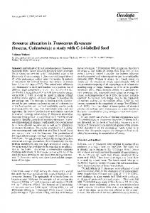
Figure 4: Scalable test problem with n “segments”.
Figure 5: (a) Value of optimal policies for the test problem; (b) Value of policies produced by the MILP approach (solid lines) and the greedy heuristic (dashed lines).
that are the main focus of this paper in that the consumption of the execution resources depends on the frequency of performing actions that utilize the resources (e.g., the more often a rover executes the “move” action, the more fuel it consumes). We can model such execution resources as follows. Let us say that whenever agent m performs action a in state i, it consumes hm ia units of an execution resource (here, for simplicity, we assume that there is only one resource, but it is trivial to extend this formulation to the case of several consumable resources). Clearly, the total expected consumption of the resource is a linear function of the occupancy measure x. Therefore, if we would like to bound the total expected use of the resource, all we have to do is add the following linear constraint to (eq. 14): XXX m ˆ hm ia xia ≤ h,
We have run two sets of experiments on two different sets of problems. One involves a scalable single-agent problem, for which it is possible to analytically compute the optimal policies. The experiments that we have performed on this set were meant to serve as a sanity check for our method, and a rough indication of how the algorithm performs under various constraint levels. We also used the single-agent problem as for our investigation of search based techniques, which we briefly report on in the next section. The second set of experiments that we have performed were done on a multiagent problem, and the main goals there were to see how the method scales with the number of agents.
m
i
a
ˆ is the upper bound on the expected resource conwhere h sumption. The ability to model linear constraints of this type is a well-known advantage of the LP formulation of MDPs (Altman 1999; Kallenberg 1983; Puterman 1994). Such linear constraints do not add to the complexity of the policy optimization problem, but they do affect the properties of optimal policies. In particular, unlike for the standard unconstrained MDPs, for the problems with such constraints, deterministic policies are no longer guaranteed to be optimal, and uniformly-optimal policies do not always exist. For some domains that involve resources whose overutilization can have dire consequences, it might not be sufficient to bound the expected consumption of a resource, and more expressive risk-sensitive constraints might be required (Ross & Chen 1988; Sobel 1985). In particular, it might be desirable to bound the probability that the resource consumption exceeds a given upper bound (Dolgov & Durfee 2003; 2004).
Empirical Evaluation and Discussion We have implemented the MILP reduction from the previous section and have run it on a series of test problems to see how it behaves. Our main goals, besides performing an empirical validation of the method, have been to see how well the algorithm scales, and also how it behaves as resource constraints are tightened or relaxed. We have also been interested in performing a preliminary investigation of searchbased methods as an alternative to the MILP approach.
Validation As a test problem for our single-agent experiments, we chose a simple problem that was easily scalable and had optimal policies whose meaning was intuitively clear. The problem is shown in Figure 4. It is composed of n twostate segments and a sink state. Thus, the problem consists of 2n + 1 states, which are numbered as shown in the figure. There are n + 1 actions, numbered from a0 to an . Action a0 is a noop that does not require any resources and can be interpreted as doing nothing. In each state si , i ∈ [1, n] (upper row), the agent can choose to execute the noop a0 and go to the next state si+1 without getting any reward. Alternatively, the agent can execute action ai that “matches” the current state, in which case it has an equal probability of either going to state sn+i (lower row) or staying in si , receiving a reward of i in both cases. However, if the agent executes any other “non-matching” action in state si , i ∈ [1, n], it goes to the sink state s0 with certainty and incurs a large penalty of −100. The only available action in states si , i ∈ [n + 1, 2n − 2] (lower row) is the noop ao , which yields a reward of zero and takes the agent to si−n+1 . There is one resource cost, and each action ai requires i units of it. For this problem the optimal policy, its value, and its resource requirements are intuitively clear and are computable analytically. In fact, this problem is equivalent to a knapsack problem where the value-to-cost ratio of all items is the same. In our experiments we varied the size of the problem (n) and the amount of the resource that was available to the agent (γ). The latter was measured as the fraction of the re-
30
80
10
CMDP joint MDP
60
10
20
time (sec)
time (sec)
25
15 10
20
10
0
10
5 0 0
40
10
−20
5
10
number of agents (n)
(a)
15
10
0
5
10
number of agents (n)
15
(b)
Figure 6: Running time of the MILP method (a), and a comparison to an optimistic estimate of the running time of the traditional “flat” multiagent MDP defined on the joint state and action spaces of all agents (b). source amount required by the optimal unconstrained policy. Figure 5a shows the value of the optimal policy as a function of γ and n. As expected, the MILP method produced the optimal policies; their values are shown in solid lines on Figure 5b. We also timed the algorithm for various constraint levels (different values of γ) and observed that the running time for highly-constrained as well as for weakly-constrained problems was significantly lower than for constraint levels in the middle range. Noting this, we constructed our multiagent test cases to have moderate constraint levels, i.e., to be the “most difficult” for our MILP method.
Scalability For our multiagent experiments, we created the following simple model of the rover domain, described in this paper’s introduction. A team of n rovers operates in an N -by-N grid world, and their task is to conduct experiments to maximize the expected scientific gain. The experiments can only be carried out at certain locations randomly placed throughout the grid. Each successfully executed experiment produces a reward, but requires a certain set of tools (determined by cm ak ). In our experiments, we limited the total amounts of tools cˆk available to the team to half of what would be needed for the optimal unconstrained policy, to represent a difficult constraint level. There is only one resource cost in this problem – each tool has a weight (specified by qk ), which is correlated with the payoff of the experiments that this tool is needed to perform; more valuable experiments require heavier tools. To avoid symmetry between the agents in our experiments, each agent was given a different load capacity (ˆ q m ) that determined how many tools the agent can carry. The big agents with high load capacities are more expensive to operate, i.e., they have higher per-move penalties than the light agents with low load capacities. The agents’ movement through the grid world has a stochastic component to it, and the agents also have a small probability of breaking down at each step. We conducted the majority of our experiments on a 10by-10 grid for various numbers of agents. Our main concern was how the solution algorithm would scale as we increased the number of agents. Figure 6a shows the running time of the MILP method (using CPLEX 8.1 on a Pentium 4 PC) for
various team sizes. The plot shows that in under 30 seconds, we could compute optimal policies for teams of 15 agents. It is interesting to contrast this result to what could have been obtained by using a traditional multiagent MDP formulated on the joint state and action spaces of all agents. It is easy to see that for this problem with 100 states, 9 actions, and 15 agents, the joint transition matrix defined on the crossproducts of the state and action spaces of all agents, would require on the order of 1074 values. Thus, it is not even possible to write down a problem of that size as a traditional multiagent MDP, let alone solve it. In fact, if we assume that for a problem with only one rover the traditional approach works a million times faster than our MILP method, and that the traditional approach scales linearly with the problem size, we can plot the running time for the two methods. Figure 6b present such a comparison graph on a logarithmic time scale, and serves as an indication of the benefits of exploiting problem structure in multiagent MDPs.
Conclusions and Future Work We have demonstrated that it can be very beneficial to “factor out” the shared resources out of the problem description and treat the resource limitations as constraints imposed on the policy optimization problem. As our analysis shows, the savings for loosely-coupled agents can be tremendous. Of course, there are many other ways of exploiting problem structure, such as abstraction (Dearden & Boutilier 1997; Boutilier, Dearden, & Goldszmidt 1995) and factorization (Boutilier, Dean, & Hanks 1999). It appears that it could be very beneficial to combine such methods with our constrained optimization approach. However, this would involve overcoming several challenges, the most important of which is probably the following. Just like the majority of methods for solving unconstrained MDPs, the existing methods that work with compact problem representations rely on Bellman’s principle of optimality, which states that the optimal action for each state is independent of the optimal actions chosen for other states. However, this principle no longer holds when global constraints are imposed on agents’ policies. Indeed, enabling an optimal action for one state might consume limited resources, making the optimal action for another state infeasible. Overcoming such difficulties in an attempt to combine compact MDP representations and our constrained optimization ideas is one of the directions of our future work. As mentioned earlier, we were also interested in exploring the possibility of using search-based methods as an alternative to the MILP approach. To this end, we compared our MILP method to a very simple heuristic search method, which worked as follows. It first solved the unconstrained problem and then sequentially replaced some actions with the noop to reduce the cost of the policy. The actions to be replaced were chosen randomly. We ran the two methods on our single-agent test problem (Figure 4). As can be seen from Figure 5b, which shows the values of the policies produced by the two methods, the greedy heuristic works very well for this test problem. This should not be surprising, given the analogy of this problem to knapsack, and the fact that all actions have the same reward-to-cost ratio. The fact
600
Policy Value
V(π)
400 200 0 −200 1
0.8
0.6
γ
0.4
0.2
0 5
10
15
20
n
Figure 7: Values of policies produced by the MILP approach (solid lines) and the greedy heuristic (dashed lines) for a slightly modified version of the problem in Figure 4.
that this elementary heuristic approach works well on some problems at a fraction of the time required for the MILP method suggests that exploring search-based approaches for this optimization problem might be worthwhile. Of course, this particular heuristic method turns out to have been well matched to this problem only by good fortune. It can do very poorly for a variation of the problem where the role of the noop and the other actions in the upper-row states si , i ∈ [1, n] is reversed. There, the noop leads to the sink state s0 , incurring a penalty of −100 and the other “nonmatching” actions lead to the next state si+1 with no reward. For this problem, the heuristic almost always produces the worst possible policy (as depicted in Figure 7). A systematic investigation of heuristic search-based methods is required before any claims can be made about the trade-offs and benefits of using such methods. This is another direction of our future work.
Acknowledgments This work was in part supported by DARPA/ITO and the Air Force Research Laboratory under contract F30602-00C-0017 as a subcontractor through Honeywell Laboratories and also through an Industrial Partners grant from Honeywell. The authors thank Kang Shin, Haksun Li, and David Musliner.
References Altman, E. 1999. Constrained Markov Decision Processes. Chapman and HALL/CRC. Bellman, R. 1957. Dynamic Programming. Princeton University Press. Boutilier, C.; Brafman, R.; and Geib, C. 1997. Prioritized goal decomposition of Markov decision processes: Towards a synthesis of classical and decision theoretic planning. In Pollack, M., ed., Proceedings of the Fifteenth International Joint Conference on Artificial Intelligence, 1156–1163. San Francisco: Morgan Kaufmann. Boutilier, C.; Dean, T.; and Hanks, S. 1999. Decisiontheoretic planning: Structural assumptions and computational leverage. Journal of Artificial Intelligence Research 11:1–94.
Boutilier, C.; Dearden, R.; and Goldszmidt, M. 1995. Exploiting structure in policy construction. In Mellish, C., ed., Proceedings of the Fourteenth International Joint Conference on Artificial Intelligence, 1104–1111. San Francisco: Morgan Kaufmann. Boutilier, C. 1999. Sequential optimality and coordination in multiagent systems. In Proceedings of the 1999 International Joint Conference on Artificial Intelligence, 478–485. Bresina, J.; Dearden, R.; Meuleau, N.; Ramkrishnan, S.; Smith, D.; and Washington, R. 2002. Planning under continuous time and resource uncertainty: A challenge for ai. In Uncertainty in Artificial Intelligence: Proceedings of the Eighteenth Conference (UAI-2002), 77–84. San Francisco, CA: Morgan Kaufmann Publishers. Dean, T., and Lin, S.-H. 1995. Decomposition techniques for planning in stochastic domains. In Proceedings of the 1995 International Joint Conference on Artificial Intelligence. Dearden, R., and Boutilier, C. 1997. Abstraction and approximate decision-theoretic planning. Artificial Intelligence 89(1-2):219–283. D’Epenoux. 1963. A probabilistic production and inventory problem. Management Science 10:98–108. Dolgov, D. A., and Durfee, E. H. 2003. Approximating optimal policies for agents with limited execution resources. In Proceedings of the Eighteenth International Joint Conference on Artificial Intelligence, 1107–1112. Dolgov, D. A., and Durfee, E. H. 2004. Approximate probabilistic constraints and risk-sensitive optimization criteria in Markov decision processes. In Proceedings of the Eighth International Symposiums on Artificial Intelligence and Mathematics (AI&M 7-2004). Garey, M. R., and Johnson, D. S. 1979. Computers and Intractability: A Guide to the Theory of NP-Completeness. W. H. Freeman & Co. Kallenberg, L. 1983. Linear Programming and Finite Markovian Control Problems. Math. Centrum, Amsterdam. Meuleau, N.; Hauskrecht, M.; Kim, K.-E.; Peshkin, L.; Kaelbling, L.; Dean, T.; and Boutilier, C. 1998. Solving very large weakly coupled Markov decision processes. In AAAI/IAAI, 165–172. Puterman, M. L. 1994. Markov Decision Processes. New York: John Wiley & Sons. Ross, K., and Chen, B. 1988. Optimal scheduling of interactive and non-interactive traffic in telecommunication systems. IEEE Transactions on Auto Control 33:261–267. Singh, S., and Cohn, D. 1998. How to dynamically merge Markov decision processes. In Jordan, M. I.; Kearns, M. J.; and Solla, S. A., eds., Advances in Neural Information Processing Systems, volume 10. The MIT Press. Sobel, M. 1985. Maximal mean/standard deviation ratio in undiscounted mdp. OR Letters 4:157–188. Wolsey, L. 1998. Integer Programming. John Wiley & Sons.