and indirect economic losses, number of endangered persons, severance of a lifeline network, etc.). Tbis lecture will first discuss in general terms how to ...
1 Optimal resource allocation for seismic reliability upgrading of existing structures and lifeline networks G. Augustia A. Borrib and M. Ciampolia a Universita di Roma 'La Sapienza', Dipartimento di lngegneria Strutturale e Geotecnica, Via Eudossiana 18; 1-00184 Roma, ltaly b Universita di Perugia, Faco1ta di Ingegneria, Via Santa Lucia Caneto1a; 1-06126 Perugia, ltaly
SUMMARY
A campaign of preventive measures aimed at upgrading an ensemble of buildings or other constructed facilities, whose seismic reliability is considered unsatisfactory, faces two difficulties: the Iimitation ofthe available resources, that must be therefore used in an optimized way, and the multiplicity ofthe aspects that should be taken into account in their allocation (direct and indirect economic losses, number of endangered persons, severance of a lifeline network, etc.). Tbis lecture will first discuss in general terms how to approach these problems (in particular how to describe the seismic vulnerability in a way that can be used in such multiobjective optimization), then will present examples of optimal allocation of the available resources to seismic upgrading of existing structures and lifelines. The examples refer to masonry buildings, whose damages can be summed with each other to obtain the total damage ofthe ensemble, and to highway networlcs, i.e., systems whose critical elements are reinforced concrete bridges. Two objective functions are considered for each example and realistic values are attributed to the relevant parameters, so that the examples confirm the feasibility and applicability of the optimal allocation. INTRODUCTION Two significant earthquakes hit ltaly in the last decades, procuring widespread damage and rnany victims: the Friuli earthquake of 1976 and the lrpinia earthquake of 1980. The epicentral area of both quakes was a rural but densely populated area, and most of the damages and victims were caused by the collapse of old masonry buildings; the disruption of the transportation networks increased much the difficulties, in particular in the latter case, also because of the collapse ofthe largest local hospital. These events spurred much research and led to widespread surveys on the vulnerability of existing buildings. Apart from the still open problems concerning the elaboration of significant statistics from the survey data, two evident difficulties now face the exploitation of the collected information to formulate a rational strategy for reduction of earthquake losses, namely: the limited amount of resources that may be available for any preventive upgrading programme, and the multiplicity of the quantities whose reduction should be pursued in any such programme, like direct and indirect economic losses, casualties and deaths, damage to artistic and cultural heritage, environmental damages, deterioration of the quality of life.
R. Rackwitz et al. (eds.), Reliability and Optimization of Structural Systems © Springer Science+Business Media Dordrecht 1995
4
Part One Keynote Lectures
This lecture will summarize a series of researches, already presented elsewhere (cf. [1-3) and the previous papers therein quoted), on the techniques that can be used to formulate and solve the problems of optimal resource allocation in a campaign for seismic risk reduction, taking account of severa) objective functions. This type of optimization, which can be a decisive help in the formulation of a rational strategy for seismic risk reduction, had previously received comparatively little attention: the aim of this lecture is not only to illustrate the problems again, but also to stimulate a discussion among specialists on structural reliability on the development and the actual exploitation of the results already obtained.
1. SEISMIC VULNERABILITY AND UPGRADING The prerequisite for the optimal allocation of the available resources is of course the availability of sufficient statistica) data on seismic vulnerability and hazard: much work has indeed be made on both these aspects in recent years. In particular, significant statistics have been and are being collected on the seismic vulnerability ofbuildings and constructed facilities, which is defined as the probability of damage under an earthquake of given intensity. Several alternative ways of describing such vulnerability exist, which can be divided into three categories. In fact, the seismic vulnerability of a structure is fully described by a set of fragility curves, that relate the probability of reaching a certain degree (or level) of damage (or a well defined limit state) with the intensity (i.e., the dangerousness) ofthe earthquake. However, due to the lack of sufficient data and the difficulties ofusing directly the fragility curves, seismic vulnerability is often measured in an approximate way by a number (the vulnerability index) or - even more simply - by including the structure in a vulnerability class. Each description has its appropriate field of application and can be associated to a different way of describing quantitatively the degree of upgrading, which is necessary for evaluating the effectiveness of preventive retrofitting measures: the three examples of optimal allocation procedures, presented in the following Sections 3 and 4, will make respectively use of each description ofvulnerability and upgrading.
1.1 Fragility curves Fragility curves require first the definition of the relevant limit state(s) or of quantitative
measures of the damage, and an analogous definition of the intensity of the action. A set of
fragility curves refers to a specific construction, and can be obtained by statistics on similar
constructions or by numerical calculations. They are therefore used for important structures: for instance, in the following they will be applied to examples of reinforced concrete girder bridges: the damage shall be measured by an indicator ofthe required ductility and ofthe energy dissipated in the critica) zones of the substructure, and the earthquake intensity by the peak ground acceleration. To evaluate the effectiveness of an upgrading intervention in this approach, a new set of fragility curves must be evaluated for the retrofitted structure, and compared with the initial one.
1.2 Vulnerability index
A set offragility curves can be replaced, in an approximate way, by a number: the vulnerability imkx, which characterizes a building without explicit reference to earthquake intensity
and level of damage. The vulnerability index can be obtained in severa) ways. For instance, G.N.D.T. (the Italian National Group for Earthquake Loss Reduction) elaborated a form, described in [4] and elsewhere, for surveying existing masonry buildings, which has experienced many variants over the years: the latest version of the form is schematically reproduced in Table 1. The survey team evaluates the quality condition of each item on a four-level scale (a); the vulnerability index is then obtained by summing up the values associated to the condition of each item, multiplied by the weights indicated in column (b): with this edition of the form, the index is comprised in the range 0-382.5, the higher values corresponding to the most vulnerable buildings.
Optimal resource allocationfor seismic reliability
5
An upgrading intervention can be defined as affecting one or more items of the form, and be assumed to bring the concemed item(s) into the best condition, i.e., to reduce to zero the contribution of that item to the vulnerability index, thus decreasing its value. In the example presented in Section 3.2 below, following previous suggestions, three possible intervention types have been defined, namely: (i) in L (light intervention) the horizontal connections between orthogonal walls are secured, thus the contribution of item 1 to the vulnerability index vanishes; (ii) M (medium intervention) includes also the strengthening of the horizontal diaphragms and brings to zero also the contribution of item 5; (iii) finally, H (heavy intervention) includes also an increase in the overall strength against horizontal actions and brings to zero the contribution of item 3. Table 1 Scheme of the survey form used lately by G.N.D. T. No. 1 2 3 4 5
6
7 8 9 10 11
Item Connection of walls Type ofwalls Total shear resistance ofwalls Soi! condition Horizontal diaphramns Plan regularity Elevation re_gularity Transverse walls: spacinw thickness Roof Non structural elements General maintenance conditions
Item condition a) Wei}!ht (b) (a) x (b) ....... 1 20 45 5 0.25 25 45 5 ······· ....... 25 45 5 1.5 ....... 0.75 25 45 5 var. 15 45 5 ······· 25 45 5 ······· 0.5 ....... 25 45 5 var. ....... 0.25 25 45 5 ....... 15 25 45 var. ....... 0.25 o 25 45 ....... 1 25 45 5 ....... Vulnerability index V
o o o o o o o o o o o
Of course, to be significative for prevision of damages and evaluation of the effectiveness of loss-reduction campaigns, the values of the vulnerability index must be calibrated versus actual damages. Such a calibration requires the definition of a measure of earthquake intensity (usually referred to a macroseismic scale) and of the degree of damage. Much work is in progress on the subject: however, the vulnerability-intensity-damage relationships are still very much affected by uncertainties, some due to incomplete calibration, some due to their inherently random nature. For simplicity's sake, in the examples presented in Section 3.2 (and in previous papers) the vulnerability index V (defined in the range 0-282, according to an earlier version ofthe survey form), the MSK earthquake intensity 1 and the degree of damage D have been assumed tobe related by the deterministic curves shown in Fig. 3, which were obtained from a statistica) analysis ofthe damages caused by some recent Italian earthquakes [5]: D =O corresponds by definition to no damage, and D = 1 to total collapse. 1.3 Damage Probability Matrices
Another definition of vulnerability assumes that aii relevant buildings can be subdivided into a lirnited (say, 3 to 5) number ofvulnerability classes, and associates each class X with a damage probability matrix (DPM). By definition, each element PiX) ofthe DPM pertaining to the vulnerability class X, is the probability that a building of that class undergoes a damage of level j, if subjected to an earthquake of intensity i. The damage of the buildings and the intensity of the earthquakes must therefore be described according to discrete scales. DPM's can be obtained from statistica! analyses of the damages due to one or more earthquake, when many buildings of a similar nature are affected, in areas of different intensities. For instance, the DPM's shown in Table 2, which are used in the example presented in Section 3.1, originated from the statistics of the damages to masonry buildings caused by the 1980 Irpinia earthquake [6): they are based on an eight-level scale of damage (ranging from no appar-
6
Part One
Keynote Lectures
ent damage to complete collapse) and detine three vulnerability classes A, B and C (A being the least safe, C the most). In Section 3.1, also a fourth ideal class D of earthquake-resistant stru~ures, including buildings which belonged to A, B, or C and have been fully upgraded, is constdered: Pji (D) = Oby assumption. Table2
Damage probability matrices, elaboratedjrom data on damages subsequent to the 1980 /rpinia earthquake [6] ClassX MSKint. i
Damage level j
1 2 3 4
5
6 7 8
6
A (worst 7
8
6
0.15 0.19 0.25 0.19 0.12 0.07 0.03 0.00
0.07 0.12 0.16 0.20 0.21 0.17 0.05 0.02
0.01 0.03 0.05 0.06 0.07 0.12 0.32 0.34
0.33 0.25 0.25 0.10 0.05 0.02 0.00 0.00
B (medium) 7 8 0.20 0.26 0.26 0.13 0.08 0.05 0.02 0.00
0.04 0.11 0.20 0.16 0.14 0.13 0.12 0.10
6 0.64 0.24 0.08 0.03 0.01 0.00 0.00 0.00
C (best 7
8
0.52 0.24 0.15 0.05 0.03 0.01 0.00 0.00
0.06 0.24 0.20 0.17 0.11 0.10 0.09 0.03
Ali significant modifications to the vulnerability of a building can be indicated by its initial and final class: e.g., AB, AC, ... BD, ... correspond to upgrading interventions, while CB, BA, CA, ... would be examples of degradation of the structure. 2. OBJECTIVES OF OPTIMIZATION
As hinted in the Introduction, any structural design and any programme of seismic loss reduction should take many aspects into account, like, e.g., economic losses, casualties and deaths, damages to the artistic and cultural heritage, environmental damages, deterioration of the quality of life. Many of these quantities are incommensurable with each other, and therefore cannot be combined into a single objective function, not even by means of weighting factors (how to weigh and compare economic costs versus human lives, or versus the destruction of a historical village?): the right approach to a rational strategy for seismic risk reduction appears to formulate and solve a problem ofmulti-objective optimal resource al/ocation. Fortunately, the objectives of the optimizations usually do not conflict with each other (a preventive intervention aimed at reducing the expected economic losses would also reduce the expected number of victims), but the respective optimal solutions - in general - do not coincide, as examples will show in the following. As discussed in Section 1 above, much research and statistica) investigations are in progress on the seismic vulnerability of existing buildings, so that the expected damage after an earthquake can be estimated. Also, many retrofitting techniques, aimed at upgrading buildings (i.e., at reducing their expected damage after an earthquake), are being developed. However, comparatively little attention has been paid - at least to the authors' knowledge to the severa! possible consequences of the damages, other than the direct economic costs: therefore, cost-benefit analyses of a campaign of preventive interventions seem possible only with reference to this aspect, and the question remains very open on how to account for the other, non-monetary aspects (often denoted intangibles) that have been quoted above. A possibility would be to correlate directly the earthquake intensity (but the same could be applied to any other environmental or man-made hazard) and each of the consequences: e.g., casualties. Not much significant work is available along these Iines, but some now begins tobe published (cf. [7]). This approach, in principle the most correct, would require specific and independent statistics for each type of consequences: and, for instance, damage statistics,
Optimal resource allocationfor seismic reliability
7
elaborated with reference to economic costs only, would be useless with regard to intangibles. On the contrary, the possibility of using the vulnerability statistics in ali cases requires that damage be defined and measured independently from the specific consequence. Other statistica) relationships should relate the damage to each relevant consequence: indeed, this approach can be applied only ifreliable damage-consequence relationships ofthis type are available [8]. In a ideal world of perfect mathematics and complete knowledge the two approaches would not differ one from the other. In the real word, they do. The great asset of the vulnerability approach lies in the unified treatment of the damage and its statistics, and in the possibility of studying the results of preventive interventions as a decrease of vulnerability, also independent of the specific consequences. Its greatest liability might appear the necessity of formulating other and separate relationships between damages and consequences, thus introducing an extra step in the calculations. But if one considers that in any case a reliable relationship between action and consequences is necessary but in many instances not (or not yet) available, it should be clear that such an approach allows to obtain al least approximate results through extrapolations of known relationships ( e.g., assume that the expected earthquake casualties in wooden buildings are sought, and that direct statistics are not available, because the specific problem was never posed before; assume also that the structural damages of timber can be forecast, and that statistics relating damages and casualties for ali buildings in the area are available: this latter statistics could be assumed valid for the wooden buildings, and introduced in the calculation ofthe expected casualties). lfthe relationship between damage and consequence is deterministic and immediate (as is implicitly assumed when no distinction is made between damage and its, say, economic cost), then the introduction ofthe extra relationship does not pose any problem whatsoever. Thus, the great liability of this approach remains in the unified quantitative definition of damage, be it made in linguistic terms (e.g., slight, significant, heavy, etc.) or in fractions or percentages (usually, O corresponds to no damage, and 100% to complete collapse; but also intermediate values, e.g. 50% or 70%, must be defined in an unequivocal way) or, perhaps better, according to a small number of damage levels. However, the vulnerability approach appears indeed essential in an optimal allocation procedure, which looks for the best distribution of the upgrading interventions, whose costs are assumed known, under a constraint on the total expenditure. In fact, it allows to calculate and introduce unified relationships between the costs of the interventions and the reduction of the vulnerability, evaluate the reduction of expected damage for each distribution of interventions, and make use ofthe relationships between damages and the consequence chosen as the objective of the optirnization in order to choose the mosi efficient o ne. In the following, it will be seen that such alternative optimizations are possible by simplified procedures or by sophisticated mathematical instruments.
3. OPTIMAL ALLOCATION OF RESOURCES: BUILDINGS 3.1 Allocation to vulnerability classes Let us start from the last (and simplest) description ofvulnerability, i.e., through DPMs. For the sake of clarity, the procedure is illustrated with direct reference to an example pertaining to masonry buildings [9], assuming the DPMs of Table 2 to hold. Realistic costs have been estimated (as percentages ofthe construction cost), both for restoring a building of each class to its original condition after a level j damage, and for each type of upgrading intervention. For simplicity's sake, ali these percentages (and the construction cost per unit building volume) have been assumed to be constant irrespective of the building volumes actually involved in the operations. The restoration costs after an earthquake of any relevant intensity can be forecast - for each class A, B and C - by multiplying the probabilities of Table 2 by the unit restoration costs estimated for each damage level, and summing up the columns: the results (again in percent of the construction cost) are shown in Table 3; small but non-zero costs, corresponding to minor
Part One Keynote Lectures
8
~nOf!. structu~) damages, have been assum~.also for the ideal class D. A preventive upgradmg mtervention changes the class of the butldmg, and therefore the forecast cost to be read in Table 3: columns (2)-(4) of Table 4 show the unit gains l>ri due to each type of intervention forecast for each given intensity i, that is, the differences between the forecast restoration cost~ without and with the interventions indicated in column (1 ).
Table3 Forecast restoration costs of masonry buildings (in percent of the construction cost)
MSKint. i ClassX
A B
c
D
7 73.3 48.8 34.7 3.30
6
56.4 41.0 30.3 0.00
8 98.3 75.8 64.0 8.30
Multiplying these forecast gains by the probabilities of occurrence 1ti of the relevant earthquake during the design life ofthe building, and summing up, the expected unit gains l>rp can be calculated. The values shown in column (5) of Table 4 have been calculated by introducing the probabilities: 1t.6 = 0.5; 1t1 = 0.2; 1t8 = 0.1; which, assuming a 100 years lifetime, correspond approximately to tne seismictty ofmany areas in Centralltaly. Table4 Forecast {5rJ and expected {5rpJ unit economic gains; cost C1 and efficiency Gc of interventions
Intervention AB
AC AD BC BD CD
Or6
15.4 26.1 56.4 10.7 41.0 30.3
Or, 24.5 38.6 70.0 14.1 45.0 31.4
Ors
22.5 34.3 90.0 11.8 67.5 55.7
Oro
14.8 24.2 51.2 9.3 36.2 27.0
C1
23.3 33.3 56.6 28.3 43.3 26.6
Gc
0.64 0.73 0.90 0.33 0.84 1.01
Finally, column (6) ofthe same Table 4 shows the assumed (deterministic) costs C1 of each intervention (once more, estimated as percentages of the construction cost), and column (7) the ratio Gc between the values in columns (5) and (6), i.e., the expected efficiency of each type of intervention. It can be noted that, with the used numerica! values (realistic, even if derived from rough estimates) most values of Gc are smaller than one, i.e., no economic advantage should be expected from preventive interventions. However, as already discussed, a number of considerations invalidates such a conclusion: it is therefore assumed that preventive interventions are actually performed and only their optimal choice is sought. (Note that, once the buildings of the examined ensemble have been assigned to a class, the procedure does not distinguish between individual buildings but can only refer to fractions of the volume of each class.) No formal optirnization procedure is necessary for the optimal choice, considering that the larger or smaller efficiency of an intervention depends on the relative values of the ratio Gc: such a comparison is easily achieved by drawing (as it bas been done in Fig. la} straight lines with slopes equal to the values of Gc. The choice of the interventions to be performed in this specific case does not present any difficulty: in fact, Fig. 1a shows immediately that the most convenient interventions are, in the order, CD, AD and BD (while in Fig. 2 a more complicated case will be found). Therefore, ifthe amount of available resources is comparatively small, they are used to bring into class D the largest possible volume of buildings belonging to class C; if more money is available than necessary to upgrade ali buildings of class C, the extra resources
Optimal resource allocation for seismic reliability
9
can be employed for intervention AD; then, if also class A can be fully upgraded, further resources can be employed for intervention BD. It is thus possible to calculate the total gain oR" = I:, orp. v,, where orP. and v, are the unit gain and the volume of each intervention, and the (o tai expenditure H = Ce· I:1(Cr V1). Examples of plots of the total gain oRp and of the volume V1 of each intervention versus the am ount of money H available for preventive upgrading are shown in Figs. lb (solid line) and le; these plots have been calculated introducing the unit construction cost: Ce = 300,000 Lire/m3, and the following volumes ofbuildings of each vulnerability class (that have been estimated for the historic centre ofPrivemo, a small medieval town approximately 100 km south ofRome [9]): VA= 441,854 m3; VB = 197,169 m3; Vc = 223,543 m3. 1.0
AB
CD AD BD AC
lirP -V1
0.8
BC 0.6 0.4
(a)
0.2
C 1 ·V 1
0.0 0.0
1.8
1.6
1.4
1.2
1.0
0.8
0.6
0.4
0.2
2.0
12
liR
100 80 60
AD
40 20
o
/'
/' /
/
/
/
/
/
/
/
/
/
/
/
/
/
/
/
/
/
/
/
/
/
/
(b)
/
_..-------- -
/
/
/
/
/
CD
o
20
H (lli'Lire) 40
60
80
100
140
120
1.0
BD
V1 (10 6 m') 0.8
AD 0.6 0.4 0.2
0.0
(c)
CD H (l0 9 Lire)
o
20
40
60
80
100
120
140
Fig. 1. Interventions distributed among building vulnerability classes, optimized with respect
to direct economic costs: (a) efficiency of interventions; (b) Expected economic gain (solid line) and comparison with the economic gain expected from the solution optimized with respect to saved lives (dotted lines); (c) interested volumes.
Part One Keynote Lectures
10
In this way, the intervention diagram, optimized with respect to the direct economic losses, has been constructed in function ofthe available resources. Table 5
Assumed ratia llj between endangered and present people
The interventions can be optimized with respect to other objectives, for instance with respect to the decrease of the number of persons endangered by an earthquake. In want of reliable models for the number of persons present and endangered by an earthquake, the calculations for this optimization have been developed assuming that (i) O. O17 persons/m3 inhabit the buildings (this value corresponds to the average density given by Italian statistics), (ii) 60% of the inhabitants are present in the buildings at the time of the earthquake, and (iii) the ratios between the number of endangered and present persons are given by Table 5 for each level of damage. Table 6
Forecast (C)nJ and expected (C)npJ number of "saved" people; cost C1and efficiency Gv of interventions Intervention
Ollt;
AB AC AD BC BD CD
0.045 0.060 0.063 0.015 0.018 0.003
Interv. substn. AB -4AC AC-4AD
on7 0.100 0.133 0.143 0.033 0.043 0.010
on8 0.321 0.419 0.549 0.098 0.228 0.130
on"
el
0.075 0.098 0.115 0.024 0.040 0.016
23.3 33.3 56.6 28.3 43.3 26.6
~l)n"
~c~
0.02~
10.0 23.3
0.017
Gv
0.00320 0.00296 0.00203 0.00084 0.00093 0.00062
Gv
0.00230 0.00073
Table 6 has been calculated in perfect analogy to Table 4. Namely, columns (2)-(4) show, for each intervention, the corresponding number 15 ni of saved people (i.e. the reduction of endangered people) per unit volume, forecast for each earthquake intensity, while column (5) shows the expected unit number 8np of saved people, assuming the already reported probabilities of occurrence. Finally, column (7) shows the efficiency of each intervention in terms of saved people, i.e. the ratio Gv between the expected unit gain of column (5) and the intervention cost of column (6): note that in the present case Gv is a ratio between two incommensurable quantities, which can be used only for comparative purposes. The last two rows of Table 6 show the differences in gains and costs between different interventions on class A, and the corresponding ratios Gv , which will be necessary to construct the optimal intervention diagram in the present case. The most convenient intervention is AB (Fig. 2a). However, if more resources are available than necessary to upgrade to class B the whole class A, it becomes next convenient not to intervene on more volumes, but to substitute intervention AC to AB: the intervention diagram is constructed as indicated in Figs. 2b and 2c, taking into account that the efficiency ofthe substitution AB -4 AC is Gv = 0.0023 (Table 6, col. 7). Ifthe whole class A can be upgraded to class C, the next convenient intervention is BD (Gv = 0.00093), then the substitution of AD to AC (Gv = 0.00073), and finally CD (Gv = 0.00062). The optimal intervention diagram is thus completed (Figs. 2b and 2c). Thus, two optimal allocations have been performed, but their objectives are not commensurable; hence, as already discussed, an overall multi-objective optimum cannot be defined.
Optimal resource allocationfor seismic reliability
11
However, the final choice ofthe solution should take into account the results ofboth calculations. To give some indications to this purpose, Figs. lb and 2b show also, in dotted Iines, respectively (Fig. 1b) the total economic gain of the solution optimized in terms of saved people, and (Fig. 2b) the people saved by the optimal economic solution. Although no general conclusions can be drawn, it can be noted that in this case the solution optimized with reference to saved people is close to optimal with respect to economic costs (Fig. lb), while the reverse is not true (Fig. 2b). BD BC
AD
0.10
CD
0.08 0.06 0.04
(a)
0.02 0.00 0.0 500
C 1 ·V 1 0.2
0.4
0.8
0.6
1.0
1.2
1.4
liNP
",-
400 300 200
100
o 1.0 0.8
______ ., / o
v. (10'
20
/
/
/
/
/
'
/
/
/
/
/
/
/
/
/
/
/
/
/
/
/
/
/
/
/
/
/
/
/
/
/
....
1.6
1.8
2.0
-- --.... .....
/
(b) H(ld' lire)
40
60
80
100
120
140 CD
n\) CD
AC-AD
AD
BD
0.6
AD
0.4
BD
0.2
(c)
H(ld'Ure) 20
40
60
80
100
120
140
Fig. 2. Interventions distributed among building vulnerability classes, optimized with respect to the decrease in the number ofpersons endangered by an earthquake (saved people): (a) efficiency of interventions; (b) expected number of saved people (solid line) and comparison with number of saved people expected from the solution optimized with respect to economic costs (dotted lines); (c) interestedvolumes.
Part One
12
Keynote Lectures
3.2 Allocation to individual buildings In this Section, the seismic vulnerability of each building is measured by a number V (the vu/nerability index) that, as anticipated in Sec.1.2, is related to the degree of damage D and the MSK earthquake intensity by the curves shown in Fig. 3. In the same Sec.1.2, three possible types of interventions (L, M and H) are defined: their assumed (deterministic) costs, together with the cost of construction, are shown in Table 7. 1.00
D
0.80
~:~V
0.60 0.40 0.20 0.00
-!=7 -7.5 I = 7.5-8
o
200
150
100
50
250
300
Fig. 3. Degree of damage D vs. vulnerability index V [5] 3.0
1.0
Ct/C
0.8
2.0
TJ
0.6 0.4
1.0
0.2 0.0
.O
.O
.O
(b)
Fig. 4. Ratios damagelconstruction costs (a) and endangeredlpresent people vs. degree of damage D (b) [10] As in Sec. 3.1, direct economic costs and number of endangered persons are taken as alternative objective functions. The assumed relationships between the degree of damage D and respectively the monetary losses and the number of endangered persons n are shown in Figs. 4a and 4b. The number ofpeople present at the moment ofthe earthquake is again assumed equal to 0.6 x 0.017 personsJm3. Table 7 Assumed construction and intervention costs per unit volume of bui/dings (Lire!m 3) Construction Ce
200 000
eL
20 000
Jntervention
L 1
CM
40,000
1
1
CH
80,000
In order to present formally the optimization problem, detine gain or re turn g~ (Ct)m of an intervention of cost C1 performed on the m-th building, the decrease in the expected damages when an earthquake ofintensity i occurs (the index k = c will indicate economic retums, k = v returns in terms of saved people). In other words, the return is equal to the difference between the damages that would occur without any intervention and after having performed the intervention of cost C1. For discrete types of interventions (like the quoted three types L, M, H), the return functions are multiple step functions.
13
Optimal resource allocationfor seismic reliability
Then, with reference to the forecast return under an earthquake of given intensity i, the optimization problem can be formulated as follows: • maximize the total return (for either k =cor k = v): Fkli{( Ct)i'( Ct)2 , •.... ,( Ct)J = LmgHCt)m
• subj ect to: N
Lm 1
(Cl)m :'> Cava
where the index m = 1, 2, ... , N indicates the building, the index i = 1, 2, 3, 4 the relevant interval of seismic intensity, and Cava is the maximum amount that can be spent in preventive interventions (available resources). The maximum can also be sought ofthe expectedtotal return: Fk = LiLm1tim gNCt)m
where 1tim is the probability ofoccurrence of an earthquake in the intensity interval i at the site of buildingm. 14
--Fc
12
------ Fv
10 8
6 4 M
2
o
o
IW~
o
M
llllli[Q]J----
1 2 3 4 5 6 7 8 9 10 ll12 13 1415 16 1718 19 20 2122 23 24 25 26 2728 29 30 Bldg.
Fig. 5. Interventions on 30 buildings, allowed by a given total amount of available resources, and optimizedwith respect to economic damages (FJ and to saved lives (Fj [10] Table 8
Assumed occurrence probabilities of earthquakes in 100 years
Buildinf[s
m- 1- 10 m-11-20 m- 21- 30
1
i MSK intensity
7-7.5
Bastia Umbra Citta di Castello Caseia
0.18 0.19 0.39
Site (town)
1tim
2
7.5-8 1t,,
0.11 0.12 0.23
3
8-8.5 1t,,
0.08 0.13 0.13
4 > 8.5 1tL[,
0.11 0.12 0.17
As already stated, the non-linearity and discontinuity of the relevant relationships do not allow the use of differential maximization procedures. But the objective functions Fk i or Fk are the sum of as many quantities as the buildings, each in turn a function of the resources assigned to the m-th building only: hence, the optimization process is a multi-stage decisional process, which can be tackled with a comparatively small number of operations by dynamic program-
14
Part One
Keynote Lectures
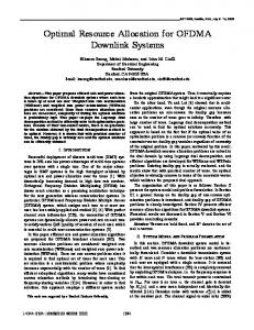
ming [10][11]. Fig. 5 shows an example of optimal allocation of 120 resource units (r.u.), with respect to Fc and to Fv, obtained by dynamic programming among 30 buildings located in three different areas of Umbria, a region of Central Italy, where the 100-year probabilities of earthquake occurrence shown in Table 8 had been approximately estimated: details on the volume and vulnerability ofthe buildings are given in [10]. 4. OPTIMAL ALLOCATION OF RESOURCES: NETWORKS AND LIFELINES 4.1 General considerations At first sight, no significant difference appears whether the optimal allocation problems presented in Section 3 refer to buildings or other facilities (e.g., bridges). But in the case ofbuildings, dealt with so far, the initial vulnerability, the consequences of failures and the benefits derived from an intervention on any element of the ensemble can be assumed - at least as a first approximation - to be independent from each other and then summable, which simplifies much the problem. On the contrary, if the facilities are elements of a system, this is no more possible: the consequences of their failure, hence the effectiveness of any preventive measure, depend not only on the vulnerabilites of the single facilities, but also in an essential way on the logica! diagram ofthe system, the critica! condition considered and the collocation (role) of each element; therefore the vulnerability of the system must be evaluated on its own account. On the other hand, it is now a well recognized fact (as very recent examples have confirmed) that the disruption of communication networks and other lifeline systems are among the most damaging effects of earthquakes. Indeed, as recent examples have confirmed, damages of this type can not only have immediate dramatic effects in the aftermath of an earthquake, but also consequences lasting for months and years on the economy, as well as on the conditions oflife, ofthe whole area affected by an earthquake (or by any other disaster). And the increasing relevance of communications and services in modem life makes these effects ali the more important. It becomes thus essential to develop the optimal allocation methodology, not only with regard to single buildings, but also to systems, and in particular lifeline networks, as first pointed out in [12]. A lifeline system can be in general modelled as a redundant network, comprising a number of vulnerable (or critica/) elements, that may themselves be complex redundant structural or mechanical systems. The network topology is usually described by its minimal cut sets or its minimal path sets, and depends on the connections between the elements and on the assumed functionality condition. From the network topology and the element vulnerabilities, it is possible to derive the reliability ofthe network as a whole. To elaborate a strategy for its improvement, it is also necessary to estimate the costs and the benefits of possible preventive measures in terms of their effects on the vulnerability of critica! elements and of the whole system. 4.2 Vulnerability of r.c. bridges As a specific, but typical, case, Section 4.3 will deal with highway networks in which, by assumption, the only vulnerable elements are the bridges. It is also assumed that the seismic vulnerability ofthe bridges is described by fragility curves, known before and after some well defined upgrading intervention. More specifically, the example bridges [2][14] are r.c. girder bridges: the decks are simply supported on piers ofhollow rectangular section (oftwo different types). Five structural diagrams have been considered (Fig. 6) in four different conditions, i.e., either as originally designed (O) for a peak ground acceleration a_g = O.lOg (in accord with the Italian Regulations), or upgraded in one of three ways, which follow two different techniques, namely: jacketing of the piers with shotcrete cover and addition of longitudinal reinforcement to improve the pier flexural capacity and shear strength (the reinforcement is increased by 50% in intervention 1; by 100% in intervention II); elimination of expansion joints between the decks and introduction of isolation/dissipation devices on piers to replace the existing bearings (intervention III).
Optimal resource allocation for seismic reliability
15
Bridgea (piers type A)
Bridge b (piers type B)
Bridge c (piers type A)
Bridged (piers type A)
Bridgee (piers type B)
Fig. 6. Structural diagrams of example bridges (measures in m) Table 9
Assumed costs of construction and of upgrading ofbridges; conditiona/ probabilities offailure of original (O) and retrofitted bridges Bridge diai!Tam onstruction cost Upgrading cost
Prlag = 0.25g
1
IT
rn o 1 II
rn
Prlag = 0.35g
o 1
IT
rn
a
b
c
d
e
56 3 4 7 3.15-10-1 2.77-1Q-1 1.94·10·1 7.29·10·3 1.00 1.00 1.00 3.02·10"2
72 6
66 3 4 9 5.60-10"1 4.71-10·1 3.49-10·1 2.66-10"3 1.00 1.00 1.00 1.14·10·2
100 7 9 14 6.29·10· 1 4.96·10-1 3.59·10·1 3.10·10·3 1.00 1.00 1.00 2.50·10·2
48 5 6 7 4.43·10·3 2.30·10-3 3.69·10·3 3.40·104 2.42·10-1 1.15-I0-1 1.22·10·1 7.57·10-3
8
9 2.82·10"1 9.62-10"2 2.71-10"2 2.33-IQ-3 1.00 8.72-10"1 4.94·10-1 1.54·10·2
The costs of construction and intervention shown in Table 9 have been assumed in the numerica! calculations: they are referred to the construction cost of bridge d, taken equal to 100 resource units (r.u.).
Part One Keynote Lectures
16
The failure condition of the bridges has been identified with the attainment of an appropriate threshold value of an indicator of the damage level in the critica! sections of the piers (as reported in detail in [14]). The fragilities of each bridge in the four conditions have been evaluated by a MonteCarlo procedure, improved by lrnportance Sampling and Directional Simulation [13], using as inputs simulated seismic accelerograms compatible with the Eurocode spectrum S2, scaled to severa! values ofthe peak ground acceleration Bg (taken as the measure of the earthquake intensity). In this way, fragility curves were plotted as functions of ~~g; the probabilities offailure ofthe five bridges corresponding to two values ofthe peak grounâ acceleration ~~g are shown in Table 9. 4.3 Optimal allocation to the criticat elements of a lifeline network The aim of the network has been identified with ensuring the connection between a source node S and a ckstination node D. Thus, the network fails when this connection is severed: this definition has obvious limitations, because many factors are not taken into account (e.g., the capacity of traftic in the emergency that foUows an earthquake), but it has been considered satisfactory for a first approach to the problem. Since the bridges are the only vulnerable elements, the network can fail only because one or more bridges fail. Only the main results of some applications are presented in the following, while for a description ofthe procedure and other details the reader is referred to [2]. The five example networks diagrammaticaly represented in Fig. 7 have been considered. Each bridge is labelled by a serial number (1-5 or 1-10) and a letter indicating the structural diagram (Fig. 6). The first network, denoted SE, is an elementary chain of elements in series, and may correspond to bridges located along a single highway stretch. It fails if any one of the bridges fail: therefore, assuming that bridge failures under a given earthquake are stochastically independent of each other, the (conditiona!) probability of network survival (1 - P80 is equal to the product of the probabilities of survival of ali elements, whence: PsE
= 1 - ~ {1 - Pi}
where Pi is the probability offailure of element i subjected to a given earthquake. The second network, denoted PA, is an elementary bundle of elements in parallel, and may represent the situation of a city cut by a river. The connection between the two banks fails if aii bridges fail, whence: PpA
=IliPi
The analogous, but more complicated, laws yielding the (conditiona!) probability of failure ofthe other networks are presented in [2] and [3]. Note that the first four networks [2] can be represented as a combination of independent subsystems in series and/or in parallel, while this is not possible for the network CO [3]. Therefore, notwithstanding the small number of nodes, this is a complex network, according to the definition given in Ref. [11], Chap. 6. Table 10 shows the failure probabilities ofthe five networks, in the original design condition (O) and after interventions of the same type on ali bridges, for two values of~ (namely 0.25 and 0.35 g, that correspond respectively to medium and high seismicity zones in Eurocode No. 8); the corresponding costs are also reported in the same table. As described in [2], resorting to dynamic programming, it is possible instead to distribute preventive upgrading interventions on the bridges in such a way that, for a given total amount of employed resources, the increase in the expected reliability after an earthquake of given intensity is maximized. The distributions of the interventions, optimized in this way for two values of !!&• are shown in Table 11, while the conditiona! failure probabilities of the networks are plotted m Fig. 8 for three values of 11g versus the amount of resources C va· The whole range of values of Cava has been investigated from nil up to the value that would allow the most efficient intervention (III) on ali bridges, i.e., 46 r.u. for the five-bridges networks, and 92 for the ten-bridges network SP2; calculations have been limited to Bg = 0.35g
Optimal resource allocation for seismic reliability
17
for the parallel network PA, because its reliability under weaker earthquakes is already very large in the original condition. NetworkSE
s
D
NetworkPA
NetworkSPJ
s
D
NetworkSP2
s
D
Network CO
s
Fig. 7. Diagrams offive example networks; locations and identijication of critica! elements With regard to the complex network CO, the optimal intervention distribution has been also obtained through an exhaustive search (in this example such a search is possible with a reasonable computational effort, because of the small number of elements). As a matter of fact, in the case of a complex network the results of the two procedures may not coincide, because in dy-
Part One Keynote Lectures
18
namic programrning the problem is analyzed by successive steps that, in this specific instance, do not correspond to independent minimal cut sets. However, the two solutions have been found identica! for all practica! purposes, being different only in the range Cava = 16- 17 r.u. for 11g = 0.25g and 11g = 0.35g: this result seems to indicate the possibility of applying the procedure based on dynamic programrning also to complex networks. Table 10 Assumed costs of retrofitting of bridges and conditiona/ probabilities of failure of original and retrofitted networks
Network Upgrading cost Prlllg = 0.25g
1
Il 111
o 1 II
111
Prlllg = 0.35g
o 1 II
111
SE 26 31 46 9.20·10"1 8.26-10"1 6.74·10·1 1.56·10·2 1.00 1.00 1.00 8.66·10"2
PA 26 31 46 1.39·104 1.43·10·5 2.43·10-6
:O
2.42·10·1 1.00-10·1 6.03·10· 1 1.00·10·9
SP1 26 31 46 6.32·10-1 4.65·10·1 3.03-10·1 7.64-lQ-3 1.00 1.00 1.00 3.82·10·2
SP2 52 62 92 5.85·10·1 3.87-10·1 2.15·10·1 1.10·10-3 1.00 1.00 1.00 2.81·10·3
co
26 31 46 3.52·10·1 7.12·10·2 1.51·10"2 2.32·10·5 1.00 9.86-10·1 7.75-10·1 6.43·104
lnspection of Fig. 8 and Table 11 can suggest many considerations. For instance, it is interesting to note how the distribution of the optimized interventions sometimes changes drastically when the amount ofthe resources varies. The convenience of an optimal versus a rule-of-thumb allocation of resources can also be put in evidence. Let for instance refer to the 10-bridge network SP2: if 11g = 0.25g and intervention II is performed on ali bridges, 62 r.u. are employed and Pris reduced from 0.58 to 0.21 ~Table 10); ifthe same 62 r.u. are distributed in the optimal way, Prbecomes as low as 0.11·10· (Fig. 8d). In the same Fig. 8d, it can be also noted that, when the resources are optimally allocated, the reduction ofPrwith Cava is very slow beyond 68 r.u.: therefore, a sensible general policy of good exploitation ofresources would allocate no more than 68 r.u. to the upgrading ofbridges in the considered network. It may be also of some interest to distinguish the preferential paths automatically chosen by the optimization procedure: in the already quoted network SP2, (6-7-8) ifCava is rather smalt, (1-4-5) ifit is larger. l.OOE+O,OJ----======::::::::=-----,
PsE
l.OOE-01
ag
=
0.15 g
(a)
Fig. 8. Probability offailure versus employed resources (optimized): a) network SE
Optimal resource allocationfor seismic reliability
19
l.OOE+OO
PpA
l.OOE-02 l.OOE-04 l.OOE-06
ag = 0.35g
l.OOE-08
(b)
I.OOE-10 l.OOE+OO
PsPt l.OOE-01
ag = 0.35g
= 0.25g l.OOE-03
(c)
l.OOE-04 l.OOE+OO
PsP2
l.OOE-02
= 0.35g llg = 0.25 g
l.OOE-04 l.OOE-06 l.OOE-08
llg = 0.15 g
o
10
20
30
40
50
60
70
80
90
(d) 100
Cava(r.u.)
l.OOE+OO
Pco
l.OOE-02 I.OOE-03 l.OOE-04 l.OOE-05 l.OOE-06 l.OOE-07 I.OOE-08 I.OOE-09
= 0.35g
= 0.25g
(e)
Fig. 8 (cont.d). Probability ofJailure versus employed resources (optimized); peak ground = 0.15g, 0.25gand 0.35g: b) network PA; c) network SPl; d) network SP2; e)
acceleration ag networkCO.
20
Keynote Lectures
Part One
Table 11
Optimized interventions on each bridge of the five example networks vs. employed resources for ag = 0.35g.
3
Cava
- - - - - - - - - - - - - - -
- - - - - - - - - - - - -
1 2 3 4 5
Cnvn
3
3
Cava
III
III III III I
III III III III
- - III III III III III III III III - - - - - - - - - - - - - - - - - - - - III III III III III III III III - - - - I III III III III III
-
- - -
-
III III III III III
III III III III I
NetworkSP1 12 15 18 21 24 27 30 33 36 39 42
9
6
- - - - -
1 2 3 4 5
1 2 3 4 5 6 7 8 9 10
III
NetworkPA 12 15 18 21 24 27 30 33 36 39 42 45 46
9
6
- - - - III III III - - - - I III III - - - - III III III - - - - III III III - - - - - - -
- - I III - III III III III III III III III - - - - III - - III III III III III III - - III III - III III III III III III III III III - - - - - - - - - - - - III III - I - - III - I III - I III III - -
1 2 3 4 5
Cava
NetworkSE 12 15 18 21 24 27 30 33 36 39 42 45 46
9
6
45 46 III III III III III
III II III III III
Network SP2 10 15 20 25 30 35 40 45 50 55 60 65 70 75 80 85 90 92
5
-
-
- - - - - - - - - - - - - - -
III III III
III III II
-
III III III
- III III III III III III III III III - - - - - - - - - - - - - - - - - - - III III III - III III III III III
-
III III III
III
- - - - - - - - III III - - - - - III - -
Cava 1 2 3 4 5
3
6
9
III
III
III II
III III
- - - - - - -
III III III III
III III III III III
-
-
III III III III III
-
III
III III III III III III
III III III III III III
III III III III III III
III -
-
III III III III III III III
III III III II III III III III III III
NetworkCO 12 15 18 21 24 27 30 33 36 39 42 45 46
- - - - - - - - III - I III III III III III III III - - - - - III III III III - - - - - - - - - - - - I - - I -
III III III
III III III
III III III
I
III
III
- - -
III III III III
III III III III
- -
III III III III I
III III III III III
III III III III III III III III III III
Optimal resource allocation for seismic reliability
21
4.4 Alternative objectives of the optimization So far, the allocation of the resources has been optimized exclusively with respect to the probability offailure ofthe network, i.e., by definition, with respect to the probability of severing the S-D connection. However, other factors should also be considered in the optirnization process: among these, the length of the time in which the network remains out of service, either after an earthquake or during the upgrading works. A first attempt at taking into consideration the time factor has been made in [3] assurning that the most efficient set of interventions is the set that yields the largest increase of reliability in the shortest time; hence, an example has been developed of an alternative optirnization of network CO, with respect to a new objective function denoted time-efficiency and equal to the ratio
AR
11 = --. T
between the variation AR of the network reliability yielded by a set of interventions and the time T* they require. The resources have then been allocated in the following way: for each ofthe paths connecting S and D, the distribution of interventions that maxirnizes the reliability of the connection in the shortest time is deterrnined; then, the path corresponding to the largest time-efficiency is selected. lf the available amount of resources is larger than the amount necessary to ensure the functionality of the most efficient path, the allocation procedure is iterated on the remaining paths. In the developed example, in this iteration both objective functions defined above have been tried: namely, the additional interventions have been planned either on the most time-efficient path among the alternative ones, or to maxirnize the further increase in the system reliability. In these cases, two alternative interventions shall appear in the relevant boxes of Table 12 (but the differences are very small). In these operations, a variant has been used ofthe algorithm first presented by Horn [15] and applied in [16] to the restoration of lifelines damaged by a seismic event. This algorithm searches in a graph the path of shortest length (of largest time-efficiency, in the present case) between S and D: this path yields the largest rate ofthe restoration curve, that is ofthe plot of the level of efficiency attained by the system (which in [16] is given by the ratio between the number ofthe restored elements and the total number of elements) versus the time needed to attain it. This path corresponds to a global optimum and does not coincide, in general, with the path obtained by choosing the optimal solution at each node of the graph. J.OOE+OO
tVTJ max 7.50E-OJ 5.00E-Ol
Path b-d
2.50E-Ol O.OOE+OO
o
15
20 cava
25
(r.u.)
Fig. 9. Network CO: Time-efficiency functions 1J versus available resources; ag
=
0.35g.
In Fig. 9 the time-efficiency functions 11 are plotted for 11g = 0.3Sg and the different paths, versus the required resources. Inspection of these plots shows that a-c is the overall most efficient path; however, at least 16 r.u. are needed for its functionality. Therefore, if a smaller
Part One Keynote Lectures
22
arnount of resources is available (but at least 6 r.u., i.e., those needed for intervention I on bridge b) the S-D connection is assured by path b-e. In deriving these plots, the time T* has been evaluated as the sum of the times needed to implement each intervention. However, similar results are obtained for the other limit case of T* equal to the longest time needed for one intervention, as if ali interventions were applied at the sarne time. The only differences appear with reference to the path b-e, because if 14 r.u. are available, an additional upgrading intervention on bridge e yields a larger increase of the efficiency than indicated by Fig. Se. The distributions of interventions, thus optimized with respect to time-efficiency, are reported in Table 12 for ag = 0.3Sg: a-c appears as the most efficient path. Note however that the probability of collapse of bridge a is very close to one both in the original state and after interventions 1 and II: hence, at least 16 r.u. are needed to ensure the functionality of the a-c path. If smaller amounts of resources are available, the optimal solution is to upgrade path b-e. Table 12. Jnterventions on each bridge (J-5) of network CO, optimized with respect to time-efficiency, vs. employed resources (3-46 r.u.) for ag = 0.35g. Cava
a b c d e
3
-
6
-
9
12
15 18 21
24 27 30 33 36 39 42 45
46 III III III III III
- - - - III III III III - - - - - - II III - - - - - - III III - - - - - - - - - - -II - - - -
III III III
III III III
III III III
III III III
III III III
III III III
1
III
III
III
III
III
- - - - - -
The thick lines in Fig. 1O show, versus the available amount of resources, the variations of the failure probability Pf of the network for three values of ag: it can be noted that the decrease ofPr is significant only beyond 16 r.u. The thin lines in the same Fig. 10 reproduce the analogous lines ofFig. Se, that correspond to a resource allocation optimized with respect to Pr: the differences between the two plots (especially significant for ag = 0.1Sg and 0.2Sg in the range 6-16 r.u.) show that optimization with respect to reliability and optimization with respect to time-efficiency lead, in general, to different sets of interventions. However, it can be noted that there are no significant differences between the two optimized allocations of an amount of resources larger than the arnount necessary to secure the functionality of at least one S-D path. l.OOE+OO .....---....
pf
l.OOE-02 l.OOE-03 l.OOE-04 l.OOE-05 l.OOE-06 l.OOE-07 l.OOE-08 l.OOE-09
Fig. 10. Probability of failure of network CO versus employed resources, optimized with respect to the time efficiency of the interventions (thick /ines) and to the network reliability (thin lines: cf Fig. 8e); peakground acceleration ag = 0.15g, 0.25gand 0.35g.
Optimal resource allocationfor seismic reliability
23
5. CONCLUDING REMARKS In Section 3, a procedure has been illustrated for the optimal allocation of the resources available for seismic upgrading of existing buildings, whose damages are assumed independent of each other. Then, Section 4 illustrates an analogous procedure for the bridges of a highway network. In this case, the reliability of the network as a system had to be considered: it has been defined as the probability that, when an earthquake of given intensity hits the area, a connection is maintained between a source and a destination node. It appears fair to say that, notwithstanding the many simplifying assumptions that have been assumed, the procedures could already be applied to real problems of resource allocation. This is true also for network optimization, at least when the reliability of the connection is the main concern. In fact, although so far only simple networks have been studied and rough quantitative estimates have been introduced, the interesting and significant results obtained appear worth further investigation. Further research is also in progress for introducing alternative objective functions ofthe optimization process of the network (like, say, the largest expected traffic capacity between source and destination after the earthquake has occurred, or the minimum repair time necessary to restore the S-D connection when it is severed as a consequence ofthe earthquake), and for taking account of severa! degrees ofdamage (ofthe elements and/or the network), implying a reduction ofload capacity ofbridges and consequently oftraffic capacity ofthe network. As a first tentative in this direction, an efficiency function defined as the ratio between the obtained increase of reliability and the time necessary to perform the upgrading interventions has been introduced in Section 4.4 as an alternative objective function. Comparing the results with those ofthe optimization with respect to reliability, it has been found that the two optimal solutions do not coincide, i.e., consideration oftime modifies the set ofinterventions tobe performed: this indicates the interest offurther studies on this problem.
ACKNOWLEDGEMENTS
This research bas been partially supported by grants from the Ministry of University and Research (M.U.R.S.T.) and from the G.N.D.T.
REFERENCES G. Augusti, A. Borri and M. Ciampoli, Seismic protection of constructed facilities: optimal use ofresources, Structural Sajety, 16(1-2) (1994) 91-102. 2. G. Augusti, A. Borri and M. Ciampoli, Optimal allocation of resources in the reduction of the seismic risk ofhighway networks, Engineering Structures, 16(7) (1994) 485-497. 3. G. Augusti and M. Ciampoli, On the seismic risk of highway networks and its reduction, Risk Analysis, Proceedings of a Symposium, Ann Arbor, Michigan (1994) 25-36. 4. G. Augusti, D. Benedetti and A. Corsanego, Investigations on seismic risk and seismic vulnerability in Italy, Proc. 4th Jnt. Conf on Structural Sajety and Reliability ICOSSAR '85, Kobe, Japan (1985) Voi. 2, 267-276. 5. D. Benedetti and G.M. Benzoni, Seismic vulnerability index versus damage for unreinforced masonry buildings, Proc. Int. Conj. on Reconstruction, Restoration and Urban Planning in Seismic prone Areas, Skopje (1985) 333-347. 6. F. Braga, M. Dolce and D. Liberatore, Southern Italy November 23, 1980 earthquake: a statistica! study on damaged buildings and an ensuing review of the MSK-76 scale, 7th European Conf on Earthquake Engineering, Athens (1982). 7. R.M. Wagner, N.P. Jones and G.S. Smith, Risk factors for casualties in earthquakes: The application of epidemiologic principles to structural engineering, Structural Safety, 13(3) (1994) 177-200. 8. G. Augusti: Discussion ofRef.[7], ibid. [in print]
1.
24 9. 10. 11. 12. 13. 14. 15. 16.
Part One Keynote Lectures G. Augusti and A. Mantuano, Sulla determînazione delia strategia ottimale per la prevenzione de! rischio sismico nei centri abitati: un nuovo approccio, L'Ingegneria Sismica in Italia 1991, Proc. 5th Italian Nat. Conj Earthquake Engrg., Palermo (1991) 117-128. G. Augusti, A. Borri and E. Speranzini, Optimum allocation of available resources to improve the reliability of building systems, Reliability and Optimization of Structural Systems '90, Proc. 3rdiFIP WG 7.5 Conference, Berkeley, California (1991) 23-32. S.S. Rao, Reliability-Based Design, McGraw-Hill, Inc. (1992). G. Augusti, A. Borri and M. Ciampoli, Optimal allocation of resources in repair and maintenance of bridge structures, Probabilistic Mechanics and Structural and Geotechnical Reliability, Proc. 6th ASCE Specialty Conf., Denver, Colorado (1992) 1-4. M. Ciampoli, R. Giannini, C. Nuti and P.E. Pinto, Seismic reliability of non-linear structures with stochastic parameters by directional simulation, Proc. 5th Intern. Conj an Structural Safety and Reliability ICOSSAR '89, S.Francisco (1989) 1121-1126. M. Ciampoli and G. Augusti, Seismic reliability assessment of retrofitted bridges, Structural Dynamics, Proc. 2d European Conference an Structural Dynamics Eurodyn '93, Trondheim, Norway (1993) Voi. 1, 193-200. W.A. Horn, Single-machine job sequencing with treelike precedence ordering and linear delay penalties, SIAM, Journal of AppliedMathematics, 23(2) (1972) 189-202. N. Nojima and H. Kameda, Optimal strategy by use oftree structures for post-earthquake restoration of lifeline network systems, Proc. Tenth World Conference an Earthquake Engineering, Madrid (1992) Voi. 9, 5541-5546.