Optimal resource allocation in synchronized multi-tier Internet services

Optimal Resource Allocation in Synchronized Multi-Tier Internet Services C. Verhoef, S. Bhulai, R.D. van der Mei

Abstract Modern Internet systems have evolved from simple monolithic systems to complex multitiered architectures. For these systems, providing good response time performance is crucial for the commercial success. In practice, the response-time performance of multi-tiered systems is often degraded by severe synchronization problems, causing jobs to wait for responses from different tiers. Synchronization between different tiers is a complicating factor in the optimal control and analysis of the performance. In this paper, we study a generic multi-tier model with synchronization. The system is able to share processing capacity between arriving jobs that need to be sent to other tiers and the responses that have arrived after processing from these tiers. We provide structural results on the optimal resource allocation policy and provide a full characterization of the policy in the framework of Markov decision theory. We also highlight important effects of synchronization in the model and discuss their implications for practice. We validate our expressions through extensive experimentations for a wide range of resource configurations. Keywords: Markov decision processes, multi-tier Internet services, optimal control, queueing networks, resource allocation, synchronization.

1

Introduction

The growing popularity of the Internet has driven the need for several businesses to open their business processes to their Web clients. Many businesses, such as retailers, auctioneers, and banks, offer significant portions of their services through the Internet. However, the computer systems that are engineered to host these applications are highly complex. Modern Internet applications have evolved from simple monolithic systems to complex multi-tiered systems. These applications do not simply deliver pre-written content but dynamically generate content on the fly using multi-tiered applications. Sometimes, these responses are generated by tens or hundreds of such multi-tiered applications. For instance, a single request to amazon.com (a major online retailer) is served by hundreds of applications operating in parallel [21]. Such elementary software applications, designed to be composed with each other, are commonly referred to as services. As shown in Figure 1, a service generates a response to each request by executing some application-specific business logic, which in turn typically issues queries to its data store and/or 1

business logic tier

client tier

data tier

request sub-services

response client synchronization and parsing

information retrieval requests

Figure 1: Application Model of an Internet Service. requests to other services. A service is exposed through well-defined client interfaces accessible over the network. Examples of services include those for processing orders and maintaining shopping carts. For online services, providing a good client experience is one of the primary concerns. Human computer interaction studies have shown that users prefer response times of less than a second for most tasks, and that human productivity improves more than linearly as computer system response times fall in the sub-second range [17]. Hence, for such online services, the design of such systems that provide low response times to their clients is a crucial business requirement. To provide good client response times, the administrators of these systems must have the ability to control its performance. In particular, one has control over the processing resources to handle jobs at different tiers. The optimal allocation of these processing resources is not trivial as different tiers are dependent on each other due to synchronization, i.e., a job cannot be further processed because it awaits answers from different tiers. For such systems, synchronization between different tiers is a complicating factor in the optimal control and analysis of the performance. In the past few years, several groups have looked at modeling Internet applications. Most of them focus on modeling single-tier applications such as Web servers [13, 8, 10, 1] and databases [5]. However, very few have studied models for multi-tier applications, like those given in Figure 1, which are more commonplace in the Web. Applying simple single-tier models to multi-tiered systems leads to poor solutions as different tiers have different characteristics. Moreover, the single-tier models do not capture the dependence between different tiers due to synchronization. In this paper we study a generic multi-tier model with synchronization in a methological framework. We provide structural results on the optimal resource allocation policy and provide a full characterization of the policy in the framework of Markov decision theory. A remarkable result is that the optimal allocation policy does not depend on the state of the sub-services in the system. We also highlight specific effects of synchronization in the model and discuss their implications for practice. We validate our expressions through extensive experimentations for a wide range of resource configurations. In contrast to most previous works on modeling Internet systems, we do not restrict ourselves to multi-tier systems with independent tiers. The rest of the paper is organized as follows. Section 2 presents the related work and Section 3 presents the system model. Section 4 presents the structural results for the optimal resource allocation policy. Section 5 highlights important effects of synchronization in the model and

2

discusses its implications for practice. Section 6 concludes the paper.

2

Related Work

2.1

Modeling Internet Systems

Various groups in the past have studied the problem of modeling Internet systems. Typical models include modeling Web servers, database servers, and application servers [13, 8, 5, 10]. For example, in [13], the authors use a queueing model for predicting the performance of Web servers by explicitly modeling the CPU, memory, and disk bandwidth in addition to using the distribution of file popularity. Bennani and Menasce [2] present an algorithm for allocating resources to a single-tiered application by using simple analytical models. Villela et al. [20] use an M/G/1/PS queueing model for business logic tiers and to provision the capacity of application servers. A G/G/1 based queueing model for modeling replicated Web servers is proposed in [19], which is to perform admission control during overloads. In contrast to these queueing based approaches, a feedback control based model was proposed in [1]. In this work, the authors demonstrate that by determining the right handles for sensors and actuators, the Web servers can provide stable performance and be resilient to unpredictable traffic. A novel approach to modeling and predicting the performance of a database is proposed in [5]. In this work, the authors employ machine learning and use an K-nearest neighbor algorithm to predict the performance of database servers during different workloads. However, the algorithm requires substantial input during the training period to perform effective prediction. All the aforementioned research efforts have been applied only to single-tiered applications (Web servers, databases, or batch applications) and do not study complex synchronized multitiered applications which is the focus of this paper. Some recent works have focused on modeling multi-tier systems. In [10], the authors model a multi-tiered application as a single queue to predict the performance of a 3-tiered Web site. As mentioned, Urgaonkar et al. [18] model multitier applications as a network of queues and assume the request flows between queues to be independent. This assumption enables them to assume a product-form network so that they can apply a mean value analysis (MVA) to obtain the mean response time to process a request in the system. Although this approach can be very effective, MVA approaches can be limiting in nature as they do not allow us to get results for the synchronized system which is of crucial importance in large scale enterprises [21].

2.2

Performance Analysis

There are few works that study the performance of Internet systems in the context of multi-tier applications. Although the response time was made explicit for the first time in [12], a lot of research on response times has already been done in other systems. Results for the business logic, modeled as a processor sharing (PS) node, are given in [6], where the Laplace-Stieltjes Transform

3

(LST) is obtained for the M/M/1/PS node. In [14] an integral representation for this distribution is derived, and in [15] the distribution is derived for the more general M/G/1/PS system (in case a representation of the service times is given). The individual services, behind the business logic, are usually modeled as first-come-first-served (FCFS) queueing systems for which results are given in [7]. The first important results for calculating response times in a queueing network are given in [9], in which product-form networks are introduced. A multi-tier system modeled as a queueing network is of product-form when the following three conditions are met. First, the arrival process is a Poisson process and the arrival rate is independent of the number of requests in the network. Second, the duration of the services (behind the business logic) should be exponentially distributed, and is not allowed to depend on the number of requests present at that service. Finally, the sequence in which the services are visited is not allowed to depend on the state of the system except for the state of the node at which the request resides. Multi-tier systems that satisfy these properties fall within the class of so-called Jackson networks and have nice properties. In [3], the authors give an overview of results on response times in queueing networks. In particular, they give expressions for the LST of the joint probability distribution for nodes which are traversed by requests in a product-form network according to a pre-defined path. Response times in a two-node network with feedback (such as at the business logic) were studied in [4]. The authors propose some solid approximations for the response times with iterative requests. They show that the approximations perform very well for the first moment of the response times. In [11], a single PS node is studied with several multi-server FCFS nodes. The authors derive exact results for the mean response time but do not allow for synchronization.

3

Problem Formulation

Consider a service system at which jobs arrive according to a Poisson process with rate λ. Upon arrival the job receives service, which has an exponentially distributed duration with parameter µa , from a server that works in a PS manner. After finishing its service, the job forks into n subjobs, and each subjob is sent to a backend server for further processing. The backend servers are modeled as single-server FIFO queues for which the service duration of backend server i is exponentially distributed with parameter µi for i = 1, . . . , n. We assume that after all subjobs of the same job have finished their service, they join back to one job; we call this synchronization. Note that jobs that have not synchronized yet, do not block the backend servers from processing other jobs, neither do they use any processing capacity in the system. The unsynchronized jobs are stored in a temporary infinitely-sized buffer until synchronization occurs. After synchronization the job is then sent back to the first PS node for its final service, which has an exponentially distributed duration with parameter µd . The system is depicted in Figure 2. The load of the PS node is defined as ρps = λ( µ1a +

1 µd ).

For backend server i the load is defined as ρi =

λ µi .

For the backend

area the load is defined as the maximum load of all backend servers, thus ρsync = max{ρ1 , ..., ρn }.

4

departures

…

PS node

…

synchronization

fork

…

arrivals

Figure 2: Model of the system In order to describe the system mathematically, we define the state space of the system as S=

= {0, 1, . . .}n+2 . An element ~s ∈ S is given by ~s = (~x, ~y ) = (xa , xd , y1 , . . . , yn ), where Nn+2 0

xa and xd represent the number of jobs in the PS node for arrival and departure, respectively, and yi represents the number of subjobs at backend node i for i = 1, . . . , n. Note that the backend node with the highest number of subjobs determines the number of forked jobs that have not synchronized yet, i.e., max{~y} = max{y1 , . . . , yn } is the number of jobs that have forked and are being processed at the backend nodes but have not synchronized yet (synchronized jobs are counted in xd ). With this description we have full information on all jobs and subjobs in the system. Based on the information ~s a controller can control the behavior of the PS node. Assuming that the capacity of the PS node is set to 1, the controller can assign a fraction a ∈ A = [0, 1] of the capacity to the xa arriving jobs and a fraction of 1 − a to the xd departing jobs. When a = xa /(xa + xd ), then the PS node shares the capacity equally among all jobs, and thus is a pure processor-sharing node. However, when the control parameter a is chosen statically we get the discriminatory processor-sharing regime. In our setting the control parameter is allowed to be dynamically set and dependent not only on the jobs in the PS node, but also on the jobs in the backend nodes. Since we want to minimize response time [17] of the multi-tier application our goal is to minimize the expected sojourn time of jobs. Minimizing the expected sojourn time corresponds to minimizing the long-run average number of jobs in the system and therefore the aim of the controller is to minimize xa + xd + max{~y}. With this description, we can fully describe the control problem as a Markov decision problem. To this end we uniformize the system (see Section 11.5 of Puterman [16]) by defining γ = λ + Pn max{µa , µd } + i=1 µi . Without loss of generality, we assume that γ = 1, since we can always get 5

this by scaling. Uniformizing is equivalent to adding dummy transitions (from a state to itself) such that the rate out of each state is equal to 1; then we can consider the rates to be transition probabilities. Let ~1 denote the vector with a 1 at all entries. Then, the transition probabilities

p, are given by p (~x, ~y), a, (xa + 1, xd , ~y) = λ for arrivals, p (~x, ~y ), a, (xa − 1, xd , ~y + ~1) = aµa if
xa > 0 for the forking of serviced arrivals, p (~x, ~y ), a, (xa , xd + max{~y} − max{~y − ei }, ~y − ei ) = µi for a service completion at backend node i for i = 1, . . . , n (note that max{~y} − max{~y − ei } checks
if synchronization has taken place), and p (~x, ~y), a, (xa , xd − 1, ~y) = (1 − a)xd for the departures.
Pn Note that due to uniformization we have p (~x, ~y), a, (~x, ~y ) = 1 − λ − aµa − (1 − a)µd − i=1 µi . Define the cost function c as c(~x, ~y ) = xa + xd + max{~y}, i.e., the number of jobs in the system. Then the tuple (S, A, p, c) fully specifies the average-cost Markov decision problem. Define a deterministic policy π as a function from S to A, i.e., π(~s) ∈ A for all ~s ∈ S. Let uπt (~s)

denote the total expected costs up to time t when the system starts in state ~s under policy

π. Note that for any stable and work-conserving policy, the Markov chain satisfies the unichain condition, so that the average expected costs g(π) = limt→∞ uπt (~s)/t is independent of the initial state ~s (see Proposition 8.2.1 of Puterman [16]). The goal is to find a policy π ∗ that minimizes the long-term average costs, thus g = minπ g(π). To determine this policy, we define V (~s) to be a real-valued function defined on the state space. This function will play the role of the relative value function, i.e., the asymptotic difference in total costs that results from starting the process in state ~s instead of some reference state. The long-term average optimal actions are a solution of the optimality equation (in vector notation) g + V = T V , where T is the dynamic programming operator acting on V defined as follows:
T V (~x, ~y) = xa + xd + max{~y} + λV (xa + 1, xd , ~y ) n + min aµa 1{xa >0} V (xa − 1, xd , ~y + ~1) + aµa 1{xa =0} V (xa , xd , ~y) a∈[0,1]

n o X

µi V (xa , xd , ~y) + (1 − a)µd V xa , (xd − 1)+ , ~y + 1 − λ − aµa − (1 − a)µd − i=1

+

n X i=1


µi V xa , xd + max{~y} − max{(~y − ei )+ }, (~y − ei )+ .

The first term in the expression T V (x) models the direct costs that are occurred per time unit. The second term deals with the arriving jobs to the system. The terms between the brackets represent the control in which the tradeoff between services of newly arrived jobs and the departing jobs is made (the fourth term between the brackets is the uniformization constant). The last term models the departures of the subjobs in the backend nodes. The optimality equation g + V = T V is usually hard to solve analytically in practice. Alternatively, the optimal actions can also be obtained by recursively defining Vl+1 = T Vl for arbitrary V0 . For l → ∞, the maximizing actions converge to the optimal ones (for existence and convergence of solutions and optimal policies we refer to Chapter 8 of Puterman [16]). This procedure is also called value iteration. We shall use this in Section 5 for the illustration of our numerical experiments. 6

4

Structural Results

In the previous section, we described the model and a solution technique to obtain the optimal policy. However, the optimal policy also possesses structural properties, which give insight into the system behaviour. In fact, in this section, we fully characterize the optimal policy as a function of the state. In order to derive these results, we reformulate the dynamic programming backward recursion equations as follows.
Vn+1 (~x, ~y) = xa + xd + max{~y} + λVn (xa + 1, xd , ~y ) + min Tna (~x, ~y) a∈[0,1]

+

n X i=1


µi Vn xa , xd + max{~y} − max{(~y − ei )+ }, (~y − ei )+ ,

with Tna (~x, ~y) = aµa 1{xa >0} Vn (xa − 1, xd , ~y + ~1) + aµa 1{xa =0} Vn (xa , xd , ~y) +

+ (1 − a)µd Vn (xa , (xd − 1) , ~y) + 1 − λ − aµa − (1 − a)µd −

n X i=1


µi Vn (xa , xd , ~y ).

We first turn our attention to the stage a job find itself in. It is intuitive to conjecture that the further a job is in its processing, the better the system is. The stages of a job can be split up into four parts (from last stage to first stage); last service by the processor-sharing node, service by the backend nodes, first service by the processor-sharing node, and arrival of a new job. In order to show that the first in the list is the best state of the system and the last in the list is the least profitable, we need to show that for arbitrary (~x, ~y ) ∈ S we have the following properties. 1. V (xa , xd , ~y) > V (xa , xd − 1, ~y) for xd > 0,
2. V (xa , xd , ~y) ≥ V xa , xd + max{~y} − max{(~y − ei )+ }, (~y − ei )+ for i = 1, . . . , N , 3. V (xa , xd , ~y) ≥ V (xa − 1, xd , ~y + ~1) for xa > 0, 4. V (xa + 1, xd , ~y) > V (xa , xd , ~y ). Note that combining the four properties above is the formalized statement of ‘the further a job is in its processing, the better the state of the system is’. In the next four lemmas, we prove the properties that are listed above. We first start with the departure of a job in the last stage: the last service by the processor-sharing node. Lemma 4.1: V (xa , xd , ~y) > V (xa , xd − 1, ~y) for all (~x, ~y) ∈ S with xd > 0. Proof : The proof is by induction on n in Vn . Define V0 (~x, ~y) = xa + xd + max{~y}. Then, clearly the statement holds. Now, assume that Vn (xa , xd , ~y ) > Vn (xa , xd − 1, ~y) for some n ∈ N. Now, we prove that Vn+1 (xa , xd , ~y) satisfies the increasingness property as well. Then, for (~x, ~y ) ∈ S with

7

xd > 0   Vn+1 (xa , xd , ~y) − Vn+1 (xa , xd − 1, ~y) = 1 + λ Vn (xa + 1, xd , ~y ) − Vn (xa + 1, xd − 1, ~y) + min Tna (xa , xd , ~y) − min Tnb (xa , xd − 1, ~y) a∈[0,1]

+

n X i=1

b∈[0,1]


 µi Vn xa , xd + max{~y} − max{(~y − ei )+ }, (~y − ei )+

− Vn xa , xd + max{~y} − max{(~y − ei )+ } − 1, (~y − ei )+




> min Tna (xa , xd , ~y) − min Tnb (xa , xd − 1, ~y). a∈[0,1]

b∈[0,1]

The equality follows by expanding Vn+1 into Vn . The inequality follows by using the induction hypothesis. Let a∗ ∈ arg mina∈[0,1] Tna Vn (xa , xd , ~y). Then, for xa > 0 ∗

∗

min Tna (xa , xd , ~y) − min Tnb (xa , xd − 1, ~y) ≥ Tna (xa , xd , ~y) − Tna (xa , xd − 1, ~y) b∈[0,1]

a∈[0,1]

  = a∗ µa Vn (xa − 1, xd , ~y + ~1) − Vn (xa − 1, xd − 1, ~y + ~1)
  + (1 − a∗ )µd Vn (xa , xd − 1, ~y) − Vn xa , (xd − 2)+ , ~y + 1 − λ − a∗ µa − (1 − a∗ )µd −

n X i=1


  µi Vn (xa , xd , ~y ) − Vn (xa , xd − 1, ~y)

≥ 0. The first inequality follows from taking a potentially suboptimal action in minb∈[0,1] Tnb (xa , xd − 1, ~y). The equality follows from the definition of Tna . The second inequality follows from the   induction hypothesis. When xa = 0, we get a∗ µa Vn (xa , xd , ~y) − Vn (xa , xd − 1, ~y) for which the induction hypothesis applies as well.

The lemma shows that a departure of the system leads to a better state of the system. This is quite intuitive since we have a job fewer in the system. We now turn our attention to the services at the backend nodes. Here, the number of jobs in the system remains the same, however, a job is closer to departure from the system. The next lemma shows that this leads to a better state as well.
Lemma 4.2: V (xa , xd , ~y) ≥ V xa , xd + max{~y} − max{(~y − ei )+ }, (~y − ei )+ for all (~x, ~y) ∈ S

and i = 1, . . . , N .

Proof : The proof is by induction on n in Vn . Define V0 (~x, ~y) = 0. Then, clearly the statement
holds. Now, assume that Vn (xa , xd , ~y ) ≥ Vn xa , xd + max{~y } − max{(~y − ei )+ }, (~y − ei )+ for all i for some n ∈

N. Now, we prove that Vn+1 (xa , xd , ~y) satisfies the property as well. Let i such

8

that yi > 0, then Vn+1 (xa , xd , ~y) − Vn+1 (xa , xd + max{~y} − max{~y − ei }, ~y − ei )   = λ Vn (xa + 1, xd , ~y ) − Vn (xa + 1, xd + max{~y} − max{~y − ei }, ~y − ei ) + min Tna (xa , xd , ~y) − min Tnb (xa , xd + max{~y} − max{~y − ei }, ~y − ei ) a∈[0,1]

+

n X j=1

b∈[0,1]


 µj Vn xa , xd + max{~y} − max{(~y − ej )+ }, (~y − ej )+

− Vn xa , xd + max{~y − ei } − max{(~y − ei − ej )+ }, (~y − ei − ej )+




≥ min Tna (xa , xd , ~y) − min Tnb (xa , xd + max{~y} − max{~y − ei }, ~y − ei ). a∈[0,1]

b∈[0,1]

The equality follows from expanding Vn+1 into Vn . The inequality follows by using the induction hypothesis. Let a∗ ∈ arg mina∈[0,1] Tna Vn (xa , xd , ~y). Then, for xa > 0 min Tna (xa , xd , ~y ) − min Tnb (xa , xd + max{~y} − max{~y − ei }, ~y − ei ) b∈[0,1]

a∈[0,1]

∗

∗

≥ Tna (xa , xd , ~y) − Tnb (xa , xd + max{~y } − max{~y − ei }, ~y − ei )   = a∗ µa Vn (xa − 1, xd , ~y + ~1) − Vn (xa − 1, xd + max{~y } − max{~y − ei }, ~y − ei + ~1)
  + (1 − a∗ )µd Vn xa , (xd − 1)+ , ~y) − Vn xa , (xd + max{~y} − max{~y − ei } − 1)+ , ~y − ei + 1 − λ − a∗ µa − (1 − a∗ )µd −

n X i=1


 µi Vn (xa , xd , ~y)

 − Vn (xa , xd + max{~y} − max{~y − ei }, ~y − ei ) . The first inequality follows from taking a potentially suboptimal action in minb∈[0,1] Tnb (xa , xd + max{~y}−max{~y −ei }, ~y −ei ). The equality follows from the definition of Tna . The second inequality follows from the induction hypothesis. Note that we used that Vn (xa − 1, xd , ~y + ~1) ≥ Vn (xa − 1, xd + max{~y +~1} − max{~y +~1− ei }, ~y − ei +~1) = Vn (xa − 1, xd + max{~y} − max{~y − ei }, ~y − ei +~1).   When xa = 0, we get a∗ µa Vn (xa , xd , ~y ) − Vn (xa , xd + max{~y } − max{~y − ei }, ~y − ei ) for which the induction hypothesis directly applies.

The proof of the lemma is somewhat more complicated, because of the max operator to count the number of jobs finished in the backend nodes. Note that the number of queues N does not play an essential role in the proof. A similar remark holds when a job is finished processing the first time at the processor-sharing node. The following lemma formalizes this. Lemma 4.3: V (xa , xd , ~y) ≥ V (xa − 1, xd , ~y + ~1) for all (~x, ~y) ∈ S with xa > 0. Proof : The proof is by induction on n in Vn . Define V0 (~x, ~y) = 0. Then, clearly the statement holds. Now, assume that Vn (xa , xd , ~y) ≥ Vn (xa − 1, xd , ~y + ~1) for some n ∈ N. Now, we prove that

9

Vn+1 (xa , xd , ~y) satisfies the property as well. Then, for (~x, ~y) ∈ S with xa > 0   Vn+1 (xa , xd , ~y ) − Vn+1 (xa − 1, xd , ~y + ~1) = λ Vn (xa + 1, xd , ~y) − Vn (xa , xd , ~y + ~1) + min Tna (xa , xd , ~y ) − min Tnb (xa − 1, xd , ~y + ~1) a∈[0,1]

+

n X i=1

b∈[0,1]


 µi Vn xa , xd + max{~y} − max{(~y − ei )+ }, (~y − ei )+

− Vn xa − 1, xd + max{~y + ~1} − max{~y + ~1 − ei }, ~y + ~1 − ei




≥ min Tna (xa , xd , ~y ) − min Tnb (xa − 1, xd , ~y + ~1) a∈[0,1]

+

n X i=1

b∈[0,1]

µi Vn xa , xd + max{~y} − max{(~y − ei )+ }, (~y − ei )+ 

− Vn xa − 1, xd + max{~y} − max{(~y − ei )+ }, ~y + ~1 − ei







≥ min Tna (xa , xd , ~y ) − min Tnb (xa − 1, xd , ~y + ~1). a∈[0,1]

b∈[0,1]

The equality follows by expanding Vn+1 into Vn . The first inequality follows by using the induction hypothesis on the terms with the arrivals. Note that we also have used the fact that max{~y + ~1} − max{~y + ~1 − ei } is equal to max{~y } − max{(~y − ei )+ } for all i. The second inequality then follows by the induction hypothesis again. Let a∗ ∈ arg mina∈[0,1] Tna (xa , xd , ~y ). Then, for xa > 1 ∗ ∗ min Tna (xa , xd , ~y) − min Tnb (xa − 1, xd , ~y + ~1) ≥ Tna (xa , xd , ~y) − Tna (xa − 1, xd , ~y + ~1)

a∈[0,1]

b∈[0,1]

 = a∗ µa Vn (xa − 1, xd , ~y + ~1) − Vn (xa − 2, xd , ~y + ~2) 

 + (1 − a∗ )µd Vn xa , (xd − 1)+ , ~y − Vn xa − 1, (xd − 1)+ , ~y + ~1 

+ 1 − λ − a∗ µa − (1 − a∗ )µd −

n X i=1


  µi Vn (xa , xd , ~y ) − Vn (xa − 1, xd , ~y + ~1)

≥ 0. The first inequality follows from taking a potentially suboptimal action in minb∈[0,1] Tnb (xa − 1, xd , ~y +~1). The equality follows from the definition of Tna . The second inequality follows from the   induction hypothesis. When xa = 1, we get a∗ µa Vn (xa −1, xd , ~y +~1)−Vn (xa −1, xd , ~y +~1) = 0. The lemma shows that when a job forks after finishing its processing at the first time it visits the processor-sharing node, the state of the system improves. It remains to show that an arrival of a job leads to a less good state of the system. The following lemma formalizes this statement. Lemma 4.4: V (xa + 1, xd , ~y) > V (xa , xd , ~y ) for all (~x, ~y) ∈ S. Proof : The proof is by induction on n in Vn . Define V0 (~x, ~y) = xa + xd + max{~y}. Then, clearly the statement holds. Now, assume that Vn (xa + 1, xd , ~y ) ≥ Vn (xa , xd , ~y ) for some n ∈ N. Now, we

10

prove that Vn+1 (~x, ~y ) satisfies the increasingness property as well. Then,   Vn+1 (xa + 1, xd , ~y ) − Vn+1 (xa , xd , ~y) = 1 + λ Vn (xa + 2, xd , ~y) − Vn (xa + 1, xd , ~y ) + min Tna (xa + 1, xd , ~y ) − min Tnb (xa , xd , ~y) a∈[0,1]

+

n X i=1

b∈[0,1]


 µi Vn xa + 1, xd + max{~y} − max{(~y − ei )+ }, (~y − ei )+

− Vn xa , xd + max{~y} − max{(~y − ei )+ }, (~y − ei )+




> min Tna (xa + 1, xd , ~y ) − min Tnb (xa , xd , ~y). a∈[0,1]

b∈[0,1]

The equality follows by expanding Vn+1 into Vn . The inequality follows by using the induction hypothesis. Let a∗ ∈ arg mina∈[0,1] Tna (xa + 1, xd , ~y ). Then, for xa > 0 ∗

∗

min Tna (xa + 1, xd , ~y) − min Tnb (xa , xd , ~y ) ≥ Tna (xa + 1, xd , ~y) − Tna (xa , xd , ~y ) b∈[0,1]

a∈[0,1]

  = a∗ µa Vn (~x, ~y + ~1) − Vn (xa − 1, xd , ~y + ~1) 

 + (1 − a∗ )µd Vn xa + 1, (xd − 1)+ , ~y − Vn xa , (xd − 1)+ , ~y + 1 − λ − a∗ µa − (1 − a∗ )µd −

n X i=1


  µi Vn (xa + 1, xd , ~y ) − Vn (xa , xd , ~y )

≥ 0. The first inequality follows from taking a potentially suboptimal action in minb∈[0,1] Tnb (xa , xd , ~y ). The equality follows from the definition of Tna . The second inequality follows from the induction   hypothesis. When xa = 0, we get a∗ µa Vn (xa , xd , ~y + ~1) − Vn (xa , xd , ~y) as first term in the equality. By applying Lemma 4.2 to Vn (xa , xd , ~y + ~1) for all i we derive that Vn (xa , xd , ~y + ~1) ≥ Vn (xa , xd + 1, ~y). By applying Lemma 4.1 subsequently, we have Vn (xa , xd , ~y + ~1) ≥ Vn (xa , xd + 1, ~y) > Vn (xa , xd , ~y), which finishes the proof. Lemmas 4.1–4.4 show that it is better to have a job further in its processing stages. This observation also suggests that the resources should be allocated such that the better stages are reached as quickly as possible. Before we turn our attention to this question, we first observe that the optimal policy allocates all resources to either the incoming or the outgoing jobs at the processor node. Lemma 4.5: The optimal policy assigns all resources to either the incoming or the outgoing jobs, i.e., arg mina∈[0,1] T a (xa , xd , ~y ) ∈ {0, 1} for all (~x, ~y ) ∈ S.

11

Proof : Note that min T a (xa , xd , ~y ) = min

a∈[0,1]

a∈[0,1]

n aµa 1{xa >0} V (xa − 1, xd , ~y + ~1) + aµa 1{xa =0} V (xa , xd , ~y)

n o X

µi V (xa , xd , ~y ) + (1 − a)µd V xa , (xd − 1)+ , ~y + 1 − λ − aµa − (1 − a)µd − i=1

= min

a∈[0,1]

n  a µa

1{xa >0} V (xa − 1, xd , ~y + ~1) + 1{xa =0} V (xa , xd , ~y ) − V (xa , xd , ~y)




+ µd V (xa , xd , ~y ) − V xa , (xd − 1)+ , ~y



o .

Now it is clear that the sign of the terms between the square brackets determines if a∗ = 0 or a∗ = 1. In particular, if xa > 0 and xd = 0, we have that V (xa − 1, xd , ~y + ~1) − V (xa , xd , ~y ) ≤ 0 (see Lemma 4.3). Hence, we have a∗ = 1. On the other, if xa = 0 and xd > 0, we have that V (xa , xd , ~y ) − V (xa , xd − 1, ~y) > 0 (see Lemma 4.1). Hence, a∗ = 0. We are now ready to prove our main theorem based on the insights obtained so far. We have already seen that based on Lemmas 4.1–4.4, the further a job is in the stage of service in the system, the better the state of the system is. Hence, based on these insights, one could conjecture that assigning all resources to the job furthest in the system might be optimal. The next theorem shows that this is indeed true and fully characterizes the optimal policy. Theorem 4.1: The optimal policy in state (~x, ~y ) ∈ S is given by a∗ =

1{xd =0} , i.e., assign all

∗

resources to the outgoing jobs if any (a = 0 when xd > 0), and assign all resources to arriving jobs otherwise (a∗ = 1 when xd = 0). Proof : In the proof of Lemma 4.5, we have already seen that if xa > 0 and xd = 0, we have that a∗ = 1. In addition, it was also shown that if xa = 0 and xd > 0, we have that a∗ = 0. Clearly, when xa = 0 and xd = 0, then a∗ = 1 is optimal (as is any other value for a∗ ). Hence, we need to show that for xa > 0 and xd > 0 we have a∗ = 0, which translates to (cf. see the proof of Lemma 4.5) showing that     µd V (xa , xd , ~y) − V (xa , xd − 1, ~y ) > µa V (xa , xd , ~y ) − V (xa − 1, xd , ~y + ~1) for all (~x, ~y) ∈ S with xa > 0 and xd > 0. The proof is by induction on n in Vn . Define V0 (~x, ~y) = 0. Then, clearly the statement holds. Now, assume that the statement holds for some n ∈ N. Now,

12

we prove that the statement also holds for n + 1. Thus,     µd V n+1 (xa , xd , ~y ) − Vn+1 (xa , xd − 1, ~y) − µa Vn+1 (xa , xd , ~y ) − Vn+1 (xa − 1, xd , ~y + ~1)   = µd (xa + xd + max{~y }) − (xa + xd + 1 + max{~y})     + µd λ Vn (xa + 1, xd , ~y) − Vn (xa + 1, xd − 1, ~y) + µd Tn∗ (xa , xd , ~y) − Tn∗ (xa , xd − 1, ~y) + µd

n X i=1


 µi Vn xa , xd + max{~y } − max{(~y − ei )+ }, (~y − ei )+


 − Vn xa , xd + max{~y} − max{(~y − ei )+ } − 1, (~y − ei )+   − µa (xa + xd + max{~y}) − (xa − 1 + xd + max{~y + ~1})     − µa λ Vn (xa + 1, xd , ~y ) − Vn (xa , xd , ~y + ~1) − µa Tn∗ (xa , xd , ~y ) − Tn∗ (xa − 1, xd , ~y + ~1) − µa

n X i=1


 µi Vn xa , xd + max{~y} − max{(~y − ei )+ }, (~y − ei )+

 − Vn (xa − 1, xd + max{~y + 1} − max{~y + ~1 − ei }, ~y + ~1 − ei ) . The equality follows from expanding Vn+1 into Vn . By rearranging terms, we find     µd V n+1 (xa , xd , ~y ) − Vn+1 (xa , xd − 1, ~y) − µa Vn+1 (xa , xd , ~y) − Vn+1 (xa − 1, xd , ~y + ~1)
 = µd + λ µd Vn (xa + 1, xd , ~y ) − Vn (xa + 1, xd − 1, ~y)
 − µa Vn (xa + 1, xd , ~y ) − Vn (xa , xd , ~y + ~1)     + µd Tn∗ (xa , xd , ~y) − Tn∗ (xa , xd − 1, ~y) − µa Tn∗ (xa , xd , ~y) − Tn∗ (xa − 1, xd , ~y + ~1) +

n X i=1


 µi µd Vn xa , xd + max{~y} − max{(~y − ei )+ }, (~y − ei )+



− Vn xa , xd + max{~y } − max{(~y − ei )+ } − 1, (~y − ei )+
− µa Vn xa , xd + max{~y} − max{(~y − ei )+ }, (~y − ei )+
 − Vn (xa − 1, xd + max{~y + ~1} − max{~y + ~1 − ei }, ~y + ~1 − ei )     > µd Tn∗ (xa , xd , ~y) − Tn∗ (xa , xd − 1, ~y) − µa Tn∗ (xa , xd , ~y) − Tn∗ (xa − 1, xd , ~y + ~1) . The inequality follows by using the induction hypothesis. Note that we also have used the fact that max{~y + ~1} − max{~y + ~1 − ei } is equal to max{~y} − max{(~y − ei )+ } for all i. First, consider

13

the case xd ≥ 2, then     µd Tn∗ (xa , xd , ~y ) − Tn∗ (xa , xd − 1, ~y) − µa Tn∗ (xa , xd , ~y) − Tn∗ (xa − 1, xd , ~y + ~1)   = µd µd Vn (xa , xd − 1, ~y) − Vn (xa , xd − 2, ~y)   − µd µa Vn (xa , xd − 1, ~y) − Vn (xa − 1, xd − 1, ~y + ~1) + µd 1 − λ − µd −

n X


  µi Vn (xa , xd , ~y ) − Vn (xa , xd − 1, ~y)

− µa 1 − λ − µd −

n X


  µi Vn (xa , xd , ~y ) − Vn (xa − 1, xd , ~y + ~1)

i=1

i=1


= µd µd Vn (xa , xd − 1, ~y) − Vn (xa , xd − 2, ~y) 


 − µa Vn (xa , xd − 1, ~y) − Vn (xa − 1, xd − 1, ~y + ~1) + 1 − λ − µd −

n X i=1



µi µd Vn (xa , xd , ~y ) − Vn (xa , xd − 1, ~y)


 − µa Vn (xa , xd , ~y ) − Vn (xa − 1, xd , ~y + ~1) ≥ 0. The first equality follows by expanding Tn∗ (~x, ~y) by taking the optimal action a∗ = 0 in the expansion. The second equality follows by rearranging the terms so that the induction hypothesis can be applied, which yields the inequality. Now, suppose that xd = 1. Recall that the uniformization Pn constant γ was defined as γ = λ + µa + µd + i=1 µi = 1. Then,     µd Tn∗ (xa , xd , ~y ) − Tn∗ (xa , xd − 1, ~y) − µa Tn∗ (xa , xd , ~y) − Tn∗ (xa − 1, xd , ~y + ~1) 

= µd µd Vn (xa , 0, ~y) + 1 − λ − µd −

n X i=1


 µi Vn (xa , 1, ~y)

n X
  µi Vn (xa , 0, ~y) − µd µa Vn (xa − 1, 0, ~y + ~1) + 1 − λ − µa − i=1

− µa µa Vn (xa − 1, 1, ~y + ~1) + 1 − λ − µa − 

+ µa µd Vn (xa − 1, 0, ~y + ~1) + 1 − λ − µd − 

n X

i=1 n X i=1


 µi Vn (xa , 1, ~y)
 µi Vn (xa − 1, 1, ~y + ~1)

= µd µd Vn (xa , 0, ~y) + µd µa Vn (xa , 1, ~y) − µd µa Vn (xa − 1, 0, ~y + ~1) − µd µd Vn (xa , 0, ~y) − µa µa Vn (xa − 1, 1, ~y + ~1) − µa µd Vn (xa , 1, ~y) + µa µd Vn (xa − 1, 0, ~y + ~1) + µa µa Vn (xa − 1, 1, ~y + ~1) = 0. The first equality follows from taking the optimal actions in the first, second and fourth term, and a suboptimal action in the third term. By rewriting all uniformization constants, we obtain the 14

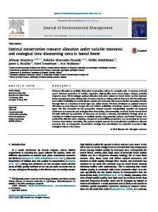
Total number of jobs at various loads 25

Varied PS arrival rate under eps policy

20 Varied PS arrival rate under dynamic policy

15

Varied PS departure rate under eps policy

10

Varied PS departure rate under dynamic policy

5

0 0.4

0.5

0.6

0.7

0.8

ߤ௔ ‫ܽߤݎ݋‬

0.9

1

Figure 3: Expected total number of jobs for different values of ρps . second equality. The previous theorem shows that the policy has a remarkably simple structure: only serve departing jobs first, and if none are available serve the newly arrived jobs first. This policy is does not take the states of the backend nodes into account. This is quite surprising, because one could expect that jobs in the backend nodes provide information to the decision maker. However, the theorem clearly shows that this intuition does not hold.

5

Numerical experiments

In the previous section, we derived structural properties of the optimal policy. The main purpose of this section is to get insight in the performance gain of the optimal policy. We numerically validate the structural results obtained in Section 4 with a broad range of parameter settings. In the following experiments we study the model as described in Section 3 with n = 2, thus we investigate the system with two backend servers in the synchronizing area. We focus on the expected total number of jobs in the system (Ltot ). For computational tractability, we truncate the state-space to 50 jobs for each dimension. This truncation at 50 jobs is high enough to obtain results that are accurate to 10−6 . In our first experiment, we study the performance of the system under different workload utilizations. We do this, by changing the parameter µa of the PS-node while keeping µd fixed, and in a different experiment, we change µd while keeping µa fixed. For both the optimal dynamic policy and under the pure processor-sharing (pps) regime (i.e., the allocation fraction a = xa /(xa + xd )), we calculate the expected total number of jobs Ltot in the system. For this purpose, let λ = 1 and µ1 = µ2 = 45 , so that ρsync = 0.8 in all cases. Figure 3 shows the results for these experiments for load values ρps that range from 0.1 to 0.95. The figure depicts four curves; the two lower curves are for the optimal policy and two upper curves are for the processor-sharing regime. For each policy, one curve depicts Ltot when µa is varied (note that µd is kept constant). For the other 15

Total number of jobs under low load 0.619

Varied PS arrival rate under eps policy

0.618

0.617

Varied PS departure rate under eps policy

0.616

0.615

Varied PS arrival rate under dynamic policy Varied PS departure rate under dynamic policy

0.614

0.613

0.612

0.611 5

6

7

8

9

10

ߤ௔ ‫ߤݎ݋‬௔

11

12

13

14

15

Figure 4: Expected total number of jobs, ρ = 0.2.

Total number of jobs under medium load 3.64

Varied PS arrival rate under eps policy

3.62 3.6

Varied PS arrival rate under dynamic policy Varied PS departure rate under eps policy

3.58 3.56 3.54 3.52 3.5

Varied PS departure rate under dynamic policy

3.48 3.46 3.44 1.8

2.3

2.8

3.3

3.8

4.3

ߤ௔ ‫ߤݎ݋‬௔

4.8

5.3

5.8

Figure 5: Expected total number of jobs, ρ = 0.6. curve, the parameter µd is varied in a similar manner. The first observation is that the dynamic policy performs better in all cases, in particular, for higher load values. The second observation, is that the system performance seems to be asymmetric, i.e., the performance of the system for a fixed (µa , µd ) is different than the performance for (µd , µa ) even though the load is the same. In order to understand the previous results more in-depth, we continue with a series of experiments in which we keep the load constant, thus we vary the parameters µa and µd such that the offered load to the system remains equal. We show that the asymmetric behavior becomes more apparent for both the optimal dynamic policy as well as the pure processor-sharing regime. The parameters for these experiments are λ = 1 and µ1 = µ2 = high loads, i.e., ρ = 0.2, 0.6, and 0.9.

16

10 9 ,

and done under low, medium, and

Total number of jobs under high load 21.00

Varied PS arrival rate under eps policy

20.50

Varied PS arrival rate under dynamic policy Varied PS departure rate under eps policy

20.00

19.50

19.00

Varied PS departure rate under dynamic policy

18.50

18.00 1

1.5

2

2.5

3

ߤ௔ ‫ߤݎ݋‬௔

3.5

4

4.5

5

Figure 6: Expected total number of jobs, ρ = 0.9. The results are shown in Figures 4–6. The figures depicts the four curves as in the previous graph; the two lower curves are for the optimal policy and two upper curves are for the processorsharing regime. For each policy, one curve depicts Ltot when µa is varied (note that µd is then completely determined, since the load is kept constant). For the other curve, the parameter µd is varied in a similar manner. In case of symmetric behaviour, the two curves should be indistinguishable from each other. However, the results show that this indeed is not the case. Under the pure processor-sharing regime this is clear for all different values of the load. In case of the optimal policy, we see that the two curves become more similar as the load increases. Next, we observe that the dynamic policy has a better performance, as predicted by our theorem, than the pure processor-sharing regime, especially under high loads. Finally, we observe that the performance is not monotone under the dynamic policy at low loads. This can be seen by the ‘W’-shape of Ltot in Figure 4. The effect diminishes as the load increases. In order to gain more insight into the performance gains of the dynamic policy versus the pure processor-sharing regime, we calculate the gain explicitly for our experiments. Table 1 shows the
percentage gain ∆ = Ltot (PPS) − Ltot (dynamic) /Ltot (P P S) for the three load cases. We can

see that one can achieve gains of 1% for low loads and almost 12% for high loads. The results in the table also suggest that when µa