Optimal Scaling of Multicommodity Flows in Wireless Ad Hoc Networks ...

Optimal Scaling of Multicommodity Flows in Wireless Ad Hoc Networks: Beyond The Gupta-Kumar Barrier Shirish Karande § , Zheng Wang § , Hamid Sadjadpour § , J.J. Garcia-Luna-Aceves §,∗ § Department of Electrical Engineering and Computer Engineering University of California, Santa Cruz, 1156 High Street, Santa Cruz, CA 95064, USA ∗ Palo Alto Research Center (PARC),3333 Coyote Hill Road, Palo Alto, CA 94304, USA Email: {karandes,wzgold,hamid,jj}@soe.ucsc.edu Abstract We establish a tight max-flow min-cut theorem for multicommodity routing in random geometric graphs. We show that, as the number of nodes in the network n tends to infinity, the maximum concurrent flow (MCF) and the minimum cut-capacity scale as Θ(n2 r3 (n)/k) for a random choice of k ≥ Θ(n) source-destination pairs, where r(n) is the communication range in the network. We exploit the fact, that the MCF in a random geometric graph equals the interference-free capacity of an ad-hoc network under the protocol model, to derive scaling laws for interferenceconstrained network capacity. We generalize all existing results reported to date by showing that the per-commodity capacity of the network scales as Θ(1/r(n)k) for the single-packet reception model suggested by Gupta and Kumar, and as Θ(nr(n)/k) for the multiple-packet reception model suggested by others. More importantly, we show that, if the nodes in the network are capable of multiple-packet transmission and reception,  then it isfeasible to achieve the optimal scaling of Θ n2 r3 (n)/k , despite the presence of interference. This result provides an improvement  of Θ nr2 (n) over the highest achieved capacity reported to date. In stark contrast to the conventional wisdom that has evolved from the Gupta-Kumar results, our results show that the capacity of ad-hoc networks can actually increase with n while the communication range tends to zero!

1 Introduction The price, performance and form factors of sensors, processors, storage elements, and radios today are at a point that the age of viable large-scale ad-hoc networks would appear to be finally upon us. Alas, Gupta and Kumar’s [8] seminal work cautions us to the contrary. They studied the capacity of wireless ad-hoc networks with n nodes when rec 1-4244-2575-4/08/$20.00 2008 IEEE

ceivers are static, transmit or receive one packet at a time, and the network traffic consists of n unicast sessions. Their conclusion was a rather negative one: The capacity of adhoc networks does not scale with an increase in network size. Gupta and Kumar’s analysis [8] applies to the traditional view of ad hoc networking in which protocols are based on a one-to-one communication paradigm aimed at avoiding multiple access interference (MAI). However, a number of recent advances in cooperative communication and generalizations of routing are challenging the long-held view that avoiding interference is the way to maximize throughput in ad hoc networks. For example, network coding (NC) [1] generalizes routing by permitting processing of packets at intermediate nodes. In certain network configurations (refer to illustrations in [9, 19]) some nodes can utilize NC to concurrently transmit multiple packets. Many-to-one and many-to-many communication is also feasible under a variety of other cooperative techniques [3, 6, 18]. Co-operative protocols that provide performance benefits in specific network configurations need not scale well with the network size. In particular, Liu et al. [15] proved another disheartening result: NC cannot increase the throughput order of wireless ad-hoc networks for multipair unicast applications under half-duplex communication. However, in a recent challenge, Garcia-Luna-Aceves et al. [6] call for the realization of ad hoc networks that scale by embracing MAI through the use of multi-packet reception (MPR) at the receivers. They show that, if the nodes in the network are capable of MPR, then the order capacity of a network with n unicast sessions grows as Θ(r(n)), where r(n)  is thecommunication range. This represents a gain of Θ nr2 (n) over the throughput order of Θ(1/nr(n)) reported by Gupta and Kumar. Interestingly, the prior work on the capacity of wireless networks, which we summarize in Section 2, has focused on what is attainable with specific approaches to handle MAI.

No prior work has focused on first establishing what is the optimal capacity of a wireless network in the absence of MAI, and then determining whether that capacity is attainable when MAI is present. This is precisely the focus and overall contribution of this paper. Section 3 presents the first contribution of this paper. We model a random network with n nodes, a homogeneous communication range of r(n), and unicast traffic for k source-destination (S-D) pairs. In the absence of interference, such a network corresponds to a random geometric graph(RGG) with an edge between any two nodes separated by a distance less than r(n). We define a combinatorial interference model based on RGGs, and use it to express all the protocol models used in the past and a model that we later use to show that the optimal capacity of a wireless network is indeed attainable. We introduce a protocol model in which nodes have the ability to decode correctly multiple packets transmitted concurrently from different nodes, and transmit concurrently multiple packets to different nodes. We refer to this as the multi-packet transmission and reception (MPTR) protocol model. Section 4 presents the second contribution of this paper, which is the characterization of the optimal interferencefree capacity of a wireless network. The task of concurrently maximizing the data-rate for k S-D pairs is an instance of the multi-commodity flow problem. Hence, the maximum concurrent multi-commodity flow-rate (MCF) in a RGG equals the interference free capacity (i.e., the optimal capacity) of the network. To derive upper bounds on the optimal network capacity, we use the fact that the MCF is less than the minimum capacity of a multi-commodity cut for any arbitrary graph. The max-flow min-cut theorem by Ford and Fulkerson [4] establishes that this bound is tight for a single commodity. However, in general, the min-cut does not provide a tight bound on the max-flow [14]. The bound is known to be tight only for special cases [10], and in general can exhibit a gap of Θ(log n) [14]. We establish a tight max-flow min-cut theorem  for RGGs for the first time,  and show that Θ n2 r3 (n)/k is a tight bound on the optimal capacity of a wireless network. Section 5 presents our third contribution, which consists of generalizing prior results by Gupta and Kumar and by Garcia-Luna-Aceves et al., and proving that the optimal capacity of wireless networks is attainable in the presence of MAI. We utilize the max-flow min-cut theorem of Section 4 to deduce tight order bounds for the capacity of random networks under various interference models. We show that the per-commodity capacity, under the protocol model suggested in [8], exhibits a tight order bound of Θ(1/r(n)k) . This result generalizes Gupta and Kumar’s result to any k ≥ Θ(n) S-D pairs. Similarly, we generalize Garcia-LunaAceves et al.’s analysis for the MPR protocol model. We show that, under the MPR model, the per-commodity ca-

pacity of the network scales as Θ(nr(n)/k), which means that itis bounded  away from the optimal capacity by a factor of Θ nr2 (n) . Furthermore, the analysis in [6] implicitly assumes the existence of a tight max-flow min-cut theorem for RGGs; therefore, the results in this paper fill an important gap in their analysis. We show that MPTR achieves the optimal capacity of Θ n2 r3(n)/k . Hence, MPTR provides a gain of Θ nr2 (n) over MPR and any previously reported feasible capacity. What is just as striking is that MPTR can achieve the dual objective of increasing capacity and decreasing the transmission range as n increases. This is in stark contrast to the commonly held view that the capacity of multihop wireless networks cannot increase as the number of nodes increases. Indeed, our results demonstrate that the capacity of ad-hoc networks can actually increase with n while the communication range tends to zero! Section 6 addresses the impact of our results on the design of protocols for future wireless ad hoc networks.

2 Related Work There have been many contributions on the capacity study of wireless ad hoc networks, however due to space limitations we only mention a few of them that focus on unicasting. A number of papers have extended the results by Gupta and Kumar [8], which showed a gap between the upper and lower bounds on capacity under the physical model. Franceschetti et al. [5] closed this gap using percolation theory. Several techniques aimed at improving the capacity of wireless ad hoc networks have been analyzed. Grossglauser and Tse [7] demonstrated that a non-vanishing capacity can be attained at the price of long delivery latencies by taking advantage of long-term storage in mobile nodes. Some works have demonstrated that changing physical layer assumptions such as using multiple channels [13] or MIMO cooperation [17] can change the network capacity. Ozgur et al. [17] proposed a hierarchical cooperation technique based on virtual MIMO to achieve linear capacity. They showed that the optimal per-session capacity of an ad-hoc network is bounded as O(n log n), and a constant per-session capacity of Θ(1) is achievable. Our work is significantly different from this work, in terms of the the model and assumptions used to derive the results. Ozgur et. al. consider the information-theoretic model, and assume that the network employs heterogenous hop-sizes, at times requiring a direct communication between widely separated nodes. In contrast, our work is based on the protocol model and assumes a homogenous transmission range, which is a more realistic assumption. Cooperation can be extended to the simultaneous transmission and reception at the various nodes in the network, which can result in significant capacity improvement [3].

As we have stated, Garcia-Luna-Aceves et al. [6] showed that using MPR at the receivers can increase the order capacity of wireless networks subject to unicast traffic. A generalization of the max-flow min-cut theorem to multiple commodities is not feasible in arbitrary graphs. However, Leighton and Rao [14] showed that the gap between the max-flow and min-cut is at most Θ(log n). In a recent work, Madan et. al. [16] have utilized the Leighton and Rao’s work to derive bounds for the capacity of ad-hoc networks. They focus on the special case where k = Θ(n2 ) and the single packet reception (SPR) model. Our work is inspired by the analysis of Leighton and Rao. Since we are able to deduce a tight max-flow min-cut theorem, our bounds are tighter than those reported by Madan et al. [16]. Furthermore, our work is applicable to a wider variety of protocol models and traffic patterns.

3 Preliminaries 3.1

Network Model

For a continuous region R, we use |R| to denote its area. We denote the cardinality of a set S by |S|, and by x − y the distance between nodes x and y. Whenever convenient, we utilize the indicator function 1{P } , which is equal to one if P is true and zero if P is false. P r(E) represents the probability of event E. We say that an event E occurs with high probability (w.h.p.) as n → ∞ if P r(E) > (1−(1/n)) . We employ the standard order notations O, Ω, and Θ. We assume a random wireless network with n nodes distributed uniformly in a unit-square. In our model, as n goes to infinity, the density of the network also goes to infinity. Therefore, our analysis is applicable to dense networks. Furthermore, we assume a fixed transmission range r(n) for all the nodes in the network. Thus, the network topology can be characterized using a RGG, which we denote by Gr and define next. Definition 3.1 Random Geometric Graph Gr : We associate a directed graph Gr (Vr , Er ) with a wireless network formed by distributing n nodes uniformly in a unit square. We represent the node-set by V = {1, · · · , n}. Let the locations of these nodes be given by {X1 , · · · , Xn }, the edge-set is then E = {(i, j) | Xi − Xj  ≤ r(n)} . While the results in this paper can be extended to undirected graphs, it is more convenient for us to use directed graphs because we use edge-coloring techniques in our work. In the case of undirected graphs, the argument should be based on vertices (receivers) rather than edges. Also note that we permit two edges for a pair of connected vertices with possibly different capacity in each direction. We assume that the network operates using a slotted channel and, in the absence of interference, the data rate

in each time slot for every transmitter-receiver pair is a constant of value W bits/slot. Given that W does not change the order capacity, we normalize its value to 1. Hence, the interference-free capacity of each edge in Gr is equal to 1. Gupta and Kumar [8] have proved the following criteria for the connectivity of Gr . Lemma 3.2 For a random distribution of n nodes in a unitsquare, the graph Gr is connected  with high probability as n → ∞, iff. r(n) ≥ rc (n) = Θ( log n/n). In a dense network, interference is the primary constraint on network capacity. Like [16], we describe the interference of a network by the following generic model. Definition 3.3 Combinatorial Interference Model: The interference model for the graph1 G(V, E) is determined by a function I : E → P (E), where P (E) is the power set of E, i.e., the set of all possible subsets of E. For every e ∈ E, I(e) represents an interference set such that, a transmission on edge e is successful if and only if (iff) there are no concurrent transmissions on any eˆ ∈ I(e). An interference model can be restricted to a sub-graph H(VH , EH ) by defining a function IH : EH → P (EH ) such that IH (e) = I(e) EH . The various protocol models that have been proposed in the past can now be expressed as special cases on Gr . Gupta and Kumar [8] studied a single packet reception (SPR) protocol model under which a transmission from node i to receiver j is successful iff Xi − Xj  ≤ r(n) and if Xj − Xk  ≥ (1 + η)r(n) for any other transmitter k. Here η is a guard-zone that is assumed to be constant for the entire network. Moreover, all the nodes operate in half-duplex mode. The following definition expresses this model in terms of the notation we have introduced. Definition 3.4 Single-Packet Reception (SPR) Model: Let e = (e+ , e− ) ∈ E, then the interference set for edge e is defined as ISPR (e) = J(e) =

J(e) − e, {ˆ e ∈ Er | Xeˆ+ − Xe−  ≤ (1 + η)r(n)}(1) .

Garcia-Luna-Aceves et al. [6] generalized the above model to account for MPR capability at the receivers. According to their MPR protocol model a node i can simultaneously receive all the packets transmitted by nodes within a distance r(n) iff there are no transmitters at a distance greater than r(n) but less than (1 + η)r(n). Furthermore, if a node j transmits a packet to node i, then it cannot simultaneously transmit a packet to any other node in the network. 1 Note

that Gr denotes a RGG while G represents a general graph.

Definition 3.5 Multi-Packet Reception (MPR) Model: IMPR (e) = A(e) = B(e) =

S-D pairs and for an arbitrary demand vector we have:

ISPR (e) − (A(e) − B(e)) ∀e ∈ E where (2) {ˆ e ∈ Er | Xeˆ+ − Xe−  ≤ r(n)}   + + eˆ ∈ Er | eˆ = e (3)

We also consider the case in which nodes have MPR and MPT capabilities, i.e., can decode multiple concurrent transmissions and can transmit concurrently multiple packets to different nodes. We capture the MPR and MPT capabilities with a simple yet representative, multi-packet transmission and reception (MPTR) protocol model, which is defined below.

lim Pr(cf (n)is feasible flow rate) =

n→∞

lim inf n→∞ Pr(c f (n)is infeasible flow rate)
0 and c < c < +∞. In the following sections we repeatedly utilize the well known Chernoff bounds: Lemma 3.9 Chernoff Bounds: Consider N i.i.d random variables Yi ∈ {0, 1} with p = Pr(Yi = 1). Let Y = N i=1 Yi . Then for every c > 0 there exist 0 < δ1 < 1 and δ2 > 0 such that

Definition 3.6 Multi-Packet Transmission and Reception (MPTR) Model: IMPTR (e) = IMPR (e) − B(e) ∀e ∈ E



Pr (Y ≤ (1 − δ1 )N p) < e−cN p Pr (Y ≥ (1 + δ2 )np) < e−cN p

(7) (8)

(4)

It is important to highlight some of the features of the above model. The MPTR protocol model still restricts the nodes to operate in a half-duplex mode. Moreover, this model is identical to the MPR protocol model in terms of the nodes that are permitted to transmit within the vicinity of a receiver i, i.e., both models prohibit transmission from a node j such that r(n) < Xi − Xj  ≤ (1 + η)r(n). Thus, the difference between the MPR and MPTR protocol models stems purely from the fact that, under the MPTR model, a node j transmitting a packet to node i can simultaneously transmit packets to other nodes in the network. We assume that the traffic in the network is generated by unicast communication between k source-destination (S-D) pairs. We associate a rate vector λ = [λ1 , · · · , λk ] with these k pairs. We assume the data rate for each S-D pair to be non-zero. Hence, without loss of generality (w.l.g) the rate vector can be written as λ = [f Di , · · · , f Dk ] where f ∈ R+ and Di ∈ [1/2, 1] for 1 ≤ i ≤ k.We refer to the parameter f as the concurrent flow rate and to D = [D1 , · · · , Dk ] as the demand vector. Definition 3.7 Feasible Flow Rate: Given k S-D pairs {(s(1), d(1)), . . . , (s(k), d(k))}, a rate vector λ = [f Di , · · · , f Dk ] is feasible if there exists a spatial and temporal scheme for scheduling transmissions such that by operating the network in a multi-hop fashion, and buffering at intermediate nodes when awaiting transmission, every source s(i) can send λi bits/sec on average to the chosen destination d(i). A flow rate f is feasible for a demand vector D = [D1 , · · · , Dk ] iff λ = [f Di , · · · , f Dk ] is a feasible rate vector. Definition 3.8 Capacity of Random Networks: The capacity per commodity of a network is Θ(f (n)) if under a random placement of n nodes,a random choice of k

3.2

Graph Theory Results

We review some definitions from graph theory. In particular, note that the task of identifying a feasible flow rate can be posed as a multi-commodity flow problem, specifically the k-commodity flow problem. Definition 3.10 k-Commodity Flow Problem: Consider a directed graph G(V, E) with a capacity function c : E → [0, 1]. Let {(s(1), d(1)), . . . , (s(k), d(k))) be k SD pairs, with a demand vector D ∈ [1/2, 1]k . Let f ∈ R+ be a concurrent flow rate. Find flow functions fi : E → R+ for 1 ≤ i ≤ k, which satisfy the following flow constraints: Capacity Constraint : ∀e ∈ E fi (e) ≤ c(e) (9) 1≤i≤k

Flow Conservation : ∀v = s(i), d(i) fi (e) = fi (e) e:e+ =v

Demand Satisfaction : 1 ≤ i ≤ k f Di = fi (e) − e:e+ =s(i)

=



e:e− =d(i)

(10)

e:e− =v



fi (e)

e:e− =s(i)

fi (e) −



fi (e)

(11)

e:e+ =d(i)

Flow functions that satisfy the above constraints are called feasible. Other inputs to the problem being fixed, a flow rate f is said to feasible iff the above problem has a solution. Furthermore, let f ∗ be the MCF such that the above problem has a feasible solution. A wireless network can be represented by an equivalent graph with capacity functions determined by the interference. Thus, the MCF in

an equivalent graph can be perceived as the maximum flow that can be routed in a network. Additionally, if w.h.p. f ∗ is the MCF for any graph formed by a random distribution of nodes, sources and destinations, then the capacity of the wireless network is also f ∗ . Consider the following additional definitions. Definition 3.11 Vertex Cut: Given a node set V , a cut is the separation of the vertex set V into two disjoint and exhaustive sets (S, S C ). We shall often reference a cut just by the set S . Definition 3.12 Multi-commodity Cut Capacity: Given a graph G(V, E), a capacity function c : E → [0, 1] and a cut (S, S C ). The multi-commodity cut capacity is defined as  e∈E 1[e+ ∈S,e− ∈S C ] c(e) (12) ΥG,S =  i:s(i)∈S,d(i)∈S C Di Definition 3.13 Minimum Cut Capacity: Given a graph G(V, E) and capacity function c : E → [0, 1], the minimum multi-commodity cut capacity is defined as ΥG = min ΥG,S (13) S⊂V

It is well-known that the minimum cut-capacity provides an upper bound on the maximum flow rate. Lemma 3.14 For any k-commodity flow f ∗ ≤ ΥG

4 Optimal Capacity We show that for RGGs, the MCF provides a tight approximation of the minimum-cut capacity. This relationship implies a tight characterization of the interference-free capacity of wireless ad-hoc networks with a homogenous transmission range. Our approach can be summarized as follows: For a particular demand vector, we provide an upper bound by showing that there exists a multi-commodity cut in Gr of order O(g(n)) and a lower bound by constructing a flow of order Ω(g(n)) in a sub-graph Hr ⊆ Gr . These results along with the following Lemmas prove that the capacity of Hr and Gr has a tight bound Θ(g(n)). Lemma 4.1 A graph G(V, E) and a sub-graph H(VH , EH ) satisfy the following two properties: (a) If f is a feasible flow-rate in H then f is feasible in G; and (b) the capacity of a cut (S, S C ) in G is always greater than or equal to the capacity of the cut in H. Proof: To prove Part (a) of the lemma, let fH,i for 1 ≤ i ≤ k be the flow functions associated with the feasible flow of rate f in H. Note that these flow functions satisfy

SS

SSc c

r(n) r(n) 2 O(nr(n) O(nr(n))2)

AA

Figure 1. A bi-partitioning of the unit square the constraints in Definition 3.10. We construct a flow in G of rate f with the following flow functions: For 1 ≤ i ≤ k let fG,i : E → R+ such that fG,i (e) = {

fH,i (e) if e ∈ EH 0 otherwise

(14)

Now, if we show that the functions fH,i satisfy the flow constraints, then the flow rate f is feasible in G. Definition 3.10 states that c(e) ≥ 0 for all the edges. As a result, ∀e ∈ E − EH the capacity constraints are satisfied trivially, given that fG,i (e) = 0 for such edges. Furthermore, ∀e ∈ EH we have fH,i (e) = fG,i (e) ≤ c(e) (15) 1≤i≤k

1≤i≤k

Therefore, fG,i satisfy the capacity constraint. In addition, note that the following equations hold ∀v ∈ V : X

X

fG,i (e) =

e∈E:e− =v

e∈EH :e− =v

=

X

fG,i (e)+

fG,i (e)

e∈E−EH :e− =v

X

fH,i (e) + 0

(16)

e∈EH :e− =v

X e∈E:e+ =v

X

fG,i (e) =

e∈EH :e+ =v

=

X

fG,i (e) +

X

fG,i (e)

e∈E−EH :e+ =v

fH,i (e) + 0

(17)

e∈EH :e+ =v

Eqs. (16) and (17) imply that the net in-flow and the net out-flow, under fG,i and fH,i , is identical for all nodes and commodities. Therefore, fG,i satisfies the flow conservation and demand constraints. To show Part (b), observe that  1[e+ ∈S,e− ∈S C ] c(e)  H (18) ΥG,S = ΥH,S + e∈E−E i:s(i)∈S,d(i)∈S C Di Since c(e) ≥ 0 for all edges, we have ΥG,S ≥ ΥH,S .



4.1

Lemma 4.3 If the network consists of k ≥ Θ(log n) S-D pairs then w.h.p. a region R of constant area |R| contains Θ(k) sources with destinations outside region R.

Upper Bound

We utilize the following properties of Gr . Lemma 4.2 If r(n) ≥ rc (n) then w.h.p. graph  Gr is such that: (a) The minimum vertex degree ∇ ≥ Θ nr2 (n) , and (b) the maximum vertex degree Δ ≤ Θ nr2 (n) .   Proof: We first show that ∇ ≥ Θ nr2 (n) . A node v in Gr is connected to all the nodes in a disk of radius r(n) centered at v . The area of this disk is πr2 (n). Given a uniformly random distribution of nodes, the probability of another node u lying within this disk is πr2 (n). Consider a random variable Yv,u ∈ {0, 1} which is equal to one iff node u is connected to node  v. The degree of node v can be written as deg(v) = u∈V −{v} Yv,u . Therefore, the Chernoff Bound (11) implies that ∀c > 0 there exists a 0 ≤ δ ≤ 1 such that   2 (19) Pr deg(v) ≤ (1 − δ)nπr2 (n) < e−cnπr (n) From the union bound we obtain   Pr ∇ ≤ (1 − δ)nπr2 (n)   < nPr deg(v) ≤ (1 − δ)nπr2 (n)

(20)

 Given that r(n) ≥ rc (n) we have r(n) ≥ c1 log n/n for some c1 > 0. Therefore, Eqs. (19) and (20) imply that   Pr ∇ ≤ (1 − δ)πnr2 (n) < ne−cπc1 log n = 1/ncπc1 −1 (21) Now, Lemma 3.9 tell us that we can choose c ≥ 2/(πc1 )) and corresponding 0 < δ1 < 1 such that   Pr ∇ ≥ (1 − δ)πnr2 (n) > 1 − (1/n) (22)  2  We use similar arguments to show that Δ ≤ Θ nr (n) w.h.p.. This fact follows from Eq. (8), which implies that ∀c > 0 there exists a 0 ≤ δ ≤ 1 such that   2 Pr deg(v) ≥ (1 + δ1 )nπr2 (n) < e−cnπr (n) (23)  The union bound and the fact that r(n) ≥ c2 log n/n implies that   Pr Δ ≥ (1 + δ)πnr2 (n) < ne−cπc2 log n (24) Therefore, there exists a δ2 > 0 s.t   Pr Δ ≤ (1 + δ2 )πnr2 (n) > 1 − (1/n)

Proof: Let Yi ∈ 0, 1 be a random variable that is equal to one iff the ith S-D pair is such that s(i) belongs to region R and d(i) does not. Under a uniformly random placement of nodes Pr (Yi = 1) = |R|(1 − |R|) (26) The total number of S-D pairs satisfying the required conk dition can be represented by Y = 1 Yi . If k ≥ c log n the Chernoff Bounds imply the existence of constants c1 = 1/(c|R|(1 − |R|)), 0 ≤ δ1 ≤ 1 and δ2 > 0 s.t. Pr (Y ≥ (1 − δ1 )|R|(1 − |R|)k) > 1 − e−c1 k|R|(1−|R|) ≥ 1 − e−c1 c|R|(1−|R|) log n = 1 − (1/n) Pr (Y ≤ (1 + δ2 )|R|(1 − |R|)k) > 1 − e

= 1 − e−c1 c|R|(1−|R|) log n = 1 − (1/n)

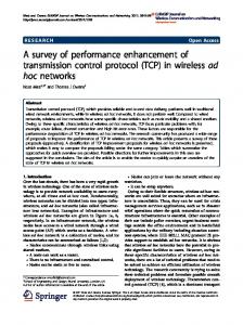
Theorem 4.4 If r(n) ≥ rc (n) and k ≥ Θ(log n), then the capacity of the cut S is ΥGr,S = O(n2 r3 (n)/k) w.h.p. Proof: According to the definition of Gr two nodes are connected iff they are separated by a distance less than r(n). Consequently, if an edge cuts across S then it has to be incident upon a node at a distance less than r(n) from the boundary separating S and S C , i.e. the head of the edge should lie in the subset A of dimension r(n) × 1. Furthermore, for each node in A the maximum number of edges cutting across the cut is bounded by Δ 1[e+ ∈S,e− ∈S C ] ≤ |A|Δ (29) e∈E

In the absence of interference c(e) = 1 for all the edges. Hence,  1[e+ ∈S,e− ∈S C ] ΥGr ,S = e∈Er i:s(i)∈S,d(i)∈S C Di |A|Δ

i:s(i)∈S,d(i)∈S C

 Consider the cut S described by Figure 1. The cut consists of all the nodes in the rectangular region of a constant area.

(28)

 Furthermore, consider the subset A in S defined by a strip of dimension 1 × r(n). The total number of vertices in A is Θ(nr(n)) because of the uniform distribution of nodes in the network.

≤  (25)

(27)

−c1 k|R|(1−|R|)

Di

(30)

According to Lemma 4.3, there exists c1 > 0 s.t. the total number S-D pairs across the cut is c1 k. Furthermore, by Definition 3.10 the demand for each pair is at least 1/2. Hence, 2|A|Δ (31) ΥGr ,S ≤ c1 k

Lemma 4.2 implies that there exists a c2 > 0 s.t. Δ < c2 nr2 (n), while uniform distribution of nodes in the network implies that there exists a c3 > 0 s.t. |A| ≤ c3 nr(n). Hence, ΥGr ,S ≤ 2c2 c3 n2 r3 (n)/(c1 k) (32)  Any cut in Gr has a capacity greater than the minimum cut capacity ΥG . Consequently Theorem 4.5 implies the following Corollary. Corollary 4.5 If r(n) ≥ rc (n) and k ≥ Θ(log n) then ΥGr is upper bounded as O(n2 r3 (n)/k).

4.2

Lower Bound

We obtain Hr by removing all edges, except those connecting two nodes in vertically or horizontally adjacent squarelets. We do not necessarily have to consider Hr in order to obtain a lower bound on the interference-free capacity. However, the performance bounds for Hr play an important role when we analyze interference constrained networks in Section 5. Definition 4.9 Geographically Restricted Sub-Graph Hr : The graph Hr (Vr , Er,H ) is a sub-graph of Gr with an identical node-set and an edge-set defined as:

l (i, j)th

i

Definition 4.8 Index Function ζ: Divide the network area into l2 squarelets [11] of sidelength a = r(n)/3 , as shown in Figure 2. Let ζ be a function that associates an index (i, j) with a squarelet in the ith column and jth row. Furthurmore, the index assigned to each squarelet is associated with each vertex in the squarelet.

square-let

Er,H = {e ∈ E | ζ(e− ) = (a, b) ⇒ ζ(e+ ) = (a±1, b±1)} (33)

h= r(n)/3 1 1

j

l

Figure 2. Decomposition of network area into l2 squarelets, each of side-length r(n)/3 25%

To describe a capacity-achieving flow in a more generic setting, we use an important result from parallel and distributed computing. Consider a mesh of l2 processing units with l processors in each row and column. Let each processor be a source and destination of exactly h packets. The problem of routing the hl2 packets to their destinations is known as h × h permutation routing and can be characterized by the following result [12]. Lemma 4.6 If in a single slot, each processor can transmit one packet each to its immediate horizontal and vertical neighbors, then an h×h permutation routing in a l ×l mesh can be performed deterministically in hl/2 + o(hl) steps. We utilize the following corollary that can be readily deduced from the above Lemma. Corollary 4.7 If a processor is capable of transmitting at least η packets to each of its neighbors in each slot, then an h × h permutation routing in a l × l mesh can be performed deterministically in O(hl/η) steps. Now consider a sub-graph Hr ⊆ Gr obtained by employing location based constraints on the edge-set. In order to describe these constraints, we first define a location dependent hash function.

r(n) 3 r(n)

Figure 3. Any two points in adjacent squarelets are within a distance r(n) of each other. The proof follows from the fact that the chord of a circle lies within it. Consider some of the properties of the squarelets and Hr . Lemma 4.10 [11] If r(n) ≥ rc (n) then w.h.p. the total number of nodes in any squarelet are Θ(nr2 (n)). Lemma 4.11 If r(n) ≥ rc (n) and k ≥ Θ(n), then w.h.p. the total number of sources in any squarelet are Θ(kr2 (n)) and the total destinations in any squarelet are Θ(kr2 (n)). Proof: For 1 ≤ i ≤ k let Yi,m ∈ 0, 1 be a random variable that is equal to one iff source s(i) belongs to the mth k squarelet. Let Ym = 1 Yi,m represent the total number of sources in the squarelet. Because r(n) ≥ rc (n), Eq.(11) implies   (34) Pr Ym ≤ (1 − δ)kr2 (n)) < e−(ck log n)/n

The total number of squarelets in a unit square is equal to (3/r(n)) × (3/r(n)) ≤ c1 n/ log n

(35)

Therefore, the union bound implies that   Pr min. no. of nodes in a squarelet < Θ(kr2 (n) ≤

(total no. of squarelets) × e−(ck log n)/n

≤ =

(c1 n/ log n) × e−(ck log n)/n c1 /(n(ck/n)−1 log n)

(36)

Thus, k ≥ Θ(n) guarantees the required convergence and hence each squarelet has at least Θ(kr2 (n)) sources. The upper bound on the number of sources and the bounds on the number of destinations can be calculated similarly.  Theorem 4.12 If r(n) ≥ rc (n) and k ≥ Θ(n),  then w.h.p. ∗ the maximum flow rate fH in Hr is at least Θ n2 r3 (n)/k . Proof: The proof follows from mapping various components of the above defined problem to the h× h permutation routing problem. Let us map each squarelet to a processor. Consequently, for the chosen size of squarelets, the network equates to a mesh of l2 processors with l = 3/r(n). Assume that each source intends to transmit Di as the ith element of the demand vector. Because Di ≤ 1, Lemma 4.11 implies that the total number of bits to be transmitted to and from each squarelet are at most h ≤ ckr2 (n). Finally, note that any two nodes in adjacent squarelets are within a distance r(n). Fig. 3 provides a geometric proof for this fact; an alternative proof can be easily obtained by employing the Pythagoras theorem. In each slot, we can send one packet along each edge between two adjacent squarelets. Therefore, Lemma 4.10 implies that η

= (min. no. of edges between adjacent squarelets) ≤ (min. no. of nodes per squarelet)2 ≤ c1 n2 r4 (n)

Hence, the total number of slots γ required to complete the desired routing is γ

≤

(c2 hl/η)

≤ =

c2 × (ckr2 (n)) × (3/r(n)) × (1/c1 n2 r4 (n)) (37) (3c2 ck/c1 n2 r3 (n))

We can repeat the above routing periodically to guarantee a flow rate of f = (1/γ) ≥ Θ(n2 r3 (n)/k). By definition, the max-flow rate is greater than any other feasible flow rate, and the theorem follows.  Aggregating the above results we have the following conclusion.  Theorem 4.13 If r(n) ≥ Θ log n/n and k ≥ Θ(n), then ∗ in Gr can be approximated tightly by the the max- flow fG ∗ min-cut capacity Υ∗Gr in Gr . Moreover, the fG and Υ∗Gr  2 3  scale as Θ n r (n)/k .

∗ ∗ ≥ fH . Hence, the Proof: Lemma 4.1 implies that fG result follows from the lower bound provided by Theorem 4.12 and the upper bound provided by Corollary 4.5.  Scaling laws for k = Θ(n) have been given special attention in the literature. Hence, it is worth stating explicitly the above results for this scenario.

Corollary 4.14 Consider an ad-hoc network described by a random placement of n nodes in a unit square, with Θ(n) S-D pairs  and a homogenous transmission range of capacity of r(n) ≥ Θ( log n/n).  The interference-free  the network scales as Θ nr3 (n) .

5 Interference-Limited Capacity 5.1

General Results

Interference can severely limit the network capacity. In this section we obtain scaling laws for the SPR, MPR and MPTR interference models. We primarily focus on deducing lower bounds. Moreover, to facilitate a succinct analysis, we develop some additional terminology and establish some important results. Recall from Section 3 that, for two different communication schemes A and B (e.g., SPR and MPR) defined in the same graph, their corresponding interference functions IA and IB are different. Definition 5.1 Dual-Interference-Set: Consider an edge set E and an interference set I(e) for an edge e ∈ E, as defined in Definition 3.3. The dual interference-set for e is defined by F (e) = {ˆ e∈ E |e ∈ I(ˆ e)}, which is the set of edges that experience a collision on account of a transmission on edge e. Definition 5.2 Dual Conflict Graph: Given a graph G(V, E) and an interference function I , we defined the dual conflict graph as GD (E, ED ) , where ED = {(e, eˆ) | eˆ ∈ I(e))}. Definition 5.3 Total Degree in Dual Conflict Graph: The total degree of each node in a dual

conflict graph is equal to |M (e)| where M (e) = I(e) F (e). Similar to the work in [16], we have the following Lemma. Lemma 5.4 Consider a graph G(V, E) and interference I. Let κ = maxe∈E |M (e)| . If f is a feasible flow rate in the absence of interference, then flow rate fI = f /(1 + κ) is feasible in presence of interference I. Proof: In the absence of interference the capacity of each edge is assumed to be one. However, because of interference, all edges cannot be activated simultaneously. Let σ

be the minimum frequency with which each edge is activated without causing any interference conflicts. Then, for each edge we have c(e) ≥ 1/σ. Observe that κ is the maximum vertex degree of the dual conflict graph GD . It is well known that, if κ is the maximum vertex degree, then κ + 1 colors are sufficient to provide a proper vertex coloring [2]. Thus, we can partition the edge-set E into 1 + κ subsets such that no two edges in the same subset interfere. Consequently, we can periodically activate these subsets to realize c(e) ≥ 1/(1 + κ) for each edge. Thus, a feasible flow rate fI = f /(1 + κ) can be obtained by scaling the flow functions associated with f by a factor of 1/(1 + κ).  The maximum vertex degree does not provide a tight bound on the minimum number of colors required to provide a proper vertex coloring. Hence, in order to analyze a wider variety of protocol models, we introduce the concept of interference clones. Definition 5.5 Interference Clone: Two edges e1 , e2 are said to be interference-clones under function I if they satisfy the conditions that M (e1 ) = M (e2 ). Lemma 5.6 Clone Piggy-backing Lemma: Consider a graph G(V, E) along with interference functions IA and IB , then IA and IB are such that: 1. κ = maxe∈E |MA (e)| 2. ∀e ∈ E there exists a set MA,B¯ (e) ⊆ MA (e) such that every edge belonging MA,B(e) is an interference-clone ¯ of e under IB . Further, let μ = mine∈E |MAB¯ (e)|. If f is a feasible flow rate in G without any interference, fIA = f /(1 + κ) is a feasible flow rate in G under the IA interference function and κ as its correponding parameter, then fIB = f (1 + μ)/(1 + κ) is feasible in presence of interference defined by IB . Proof: Consider the interference defined by IA . From Lemma 5.4 we know that there exists a conflict free periodic schedule which can activate each edge at least once every (1 + κ) slots. Let us represent this schedule by an indicator function α(e, τ ) which equals one iff edge e is active in slot τ . Note that the capacity of each edge under schedule α is given by cα (e) = Στ α(e, τ ) = 1/(1 + κ).

(38)

Now let us use this schedule in the presence of interference IB . Observe that, for every  e, α allocates a distinct slot for each edge in MA,B¯ (e) {e}. Consequently, every edge has |MA,B¯ (e)| interference clones scheduled in slots distinct from each other and the edge itself. In addition, note that if an edge is activated in a time slot meant for one of

its interference clones, then it does not lead to any conflict. Therefore, we can define a new conflict-free schedule  β such that β(e, τ ) = 1 iff there exits an e1 ∈ MA,B¯ (e) {e} such that α(e1 , τ ) = 1. Given that μ = mine∈E |MAB¯ (e)|, the capacity of each edge under schedule β for interference IB , is given by cβ (e) = Σe1 ∈MA,Bˆ Στ α(e1 , τ ) ≤ (1 + μ) × (1/(1 + κ))

(39)

Accordingly, a feasible flow of fIB = f (1 + μ)/(1 + κ) can be obtained by scaling all the flow functions associated with the inference-free flow by a factor of (1+μ)  (1+κ) . In the subsequent discussion, we find it convenient to deduce a bound for a particular interference model and then show that it applies to a wider set of models. In order to facilitate such arguments, we define the following partial order. Definition 5.7 Partial Order of Interference Models: An interference function IA is said to be more restrictive than IB , represented as IA IB , iff every edge satisfies the conditions that IB (e) ⊆ IA (e) . Lemma 5.8 Consider a graph G(V, E) along with interference IA and IB . If IA IB , then a feasible flow rate under IA remains feasible under IB . Proof: A conflict free schedule under IA remains conflict free under IB . Hence we can say that cA (e) ≤ cB (e)

(40)

where cA (e) and cB (e) represent the edge capacities under each interference model. Therefore, if a particular flow satisfies the capacity constraints under IA , it necessarily satisfies those same constraints under IB . 

5.2

Lower Bounds

Direct analysis of the interference models can be tedious. Hence, for mathematical convenience, we consider the following restrictive models. Lemma 5.8 allows us to utilize the performance limits under these restrictive models to indirectly bind the capacity under the interference models for SPR, MPR and MPTR. We define a restrictive interference model that introduces more restrictions (i.e., collisions) on the interference set for each edge than those strictly dictated by the original interference model. We will show that, under this restrictive model, the order of the lower bound capacity achieves the upper bound under the original (non-restrictive) interference model.

Definition 5.9 Restricted SPR (RSPR) Model: IRSPR (e) = where W (e) =

W (e) − {e} ∀e ∈ Er,H  MSP R (ˆ e)

(41)

a node v such that r(n) < Xe− − Xv  ≤ (1 + η)r(n). Therefore, there exists an annular ring around e− of width ηr(n) such that any transmission from a node in this ring interferes with e. The area of this annular ring is given by area of annular ring = η(2 + η)πr2 (n)

eˆ:ζ(ˆ e− )=ζ(e− )

We have already seen ( Lemma 4.2) that an area of Θ(r2 (n)) contains at least Θ(nr2 (n)) nodes. Hence, there exists a c3 such that

Definition 5.10 Restricted MPR (RMPR) Model: = W (e) − U (e) ∀e ∈ Er,H   where U (e) = eˆ ∈ Er,H | eˆ− = e−

IRMPR (e)

(42)

Definition 5.11 Restricted MPTR (RMPTR) Model: IRMPTR (e) where V (e)

= W (e) − V (e) ∀e ∈ Er,H  = U (ˆ e)

(43)

eˆ:ζ(ˆ e− )=ζ(e− )

Consider the following properties of the restricted models. Lemma 5.12 For the graph Hr , we have a partial order defined by (i) ISPR IMPR IMPTR , (ii) IRSPR IRMPR IRMPTR , (iii) ISPR IRSPR (iv) IRMPR IMPR (v) IRMPTR IMPTR Proof: (Sketch) The proof for the partial orders (i) to (iii) follows directly from the definitions. Partial order (iv) follows from the fact that J(e) ⊆ W (e) and U (e) ⊆ A(e) − B(e). Similarly, the fact that A(e) ⊆ V (e) implies partial order (v).  Lemma 5.13 If r(n) ≥ rc (n), then all edges e ∈ Er,H have |M (e)| = Θ n2 r4 (n) under interference described by either of the models: ISPR , IMPR , IMPTR , IRSPR , IRMPR , IRMPTR . Proof: From Lemma 5.12 we can conclude that RSPR is the most restrictive model, while MPTR is the least restrictive model. Further note that FRSPR (e) ⊆ W (e) and IMPTR (e) ⊆ MMPTR (e). Hence, it suffices to prove the following: γmax = maxe∈Er,H |W (e)| = O(n2 r4 (n))

(44)

γmin = mine∈Er,H |IMPTR (e)| = Ω(n2 r4 (n))

(45)

Recall that a node in Hr is connected to all and only those nodes that are placed in adjacent squarelets. Hence Lemma 4.10 tells us that the degree of each vertex v ∈ Hr is bounded as 4c1 nr2 (n) ≤ deg(v) ≤ 4c2 nr2 (n)

(47)

(46)

Now lets prove the lower bound by considering the model MPTR. According to Definition 3.6, the transmission on edge e experiences interference from any transmission by

γmin ≥ c3 nr2 (n) × 4c1 nr2 (n)

(48)

Eq. (48) proves the reqd. lower bound. The proof for the upper bound is obtained with a similar argument. First, let us inspect the transmission along edge e under the SPR model. Any transmission from a node in a disk of radius (1 + η)r(n) around e− , interferes with e. Moreover, a transmission from e+ interferes with any reception in a disk of radius (1 + η)r(n) around e+ . Given that Xe+ − Xe−  ≤ r(n), there exists a disk of radius (2 + η)r(n) around e− containing all the nodes that may have transmission conflicts with e. Further note that a squarelet can √ be completely inscribed in a circum-circle of radius (1/3 2)r(n). Hence, there √ exists a circle of maximum radius R = (2 + η + (1/3 2))r(n) containing all the nodes that may have transmission conflicts with e under the model RSPR. The area of R is Θ(r2 (n)) and hence there exists a constant c4 such that γmax

=

maxe∈Er,H |W (e)|

≤ ≤

(max. no. of nodes in R) × (max. node degree) √ c4 n(2 + η + ( 2/6))2 r(n)2 × 4c2 nr2 (n)

=

O(n2 r4 (n))

(49) 

Lemma 5.14 Consider the graph Hr with r(n) ≥ rc (n) and k ≥  Θ(n).  In such a graph, each edge e has at least Θ nr2 (n) clones under interference IRMPR and Θ n2 r4 (n) clones under interference IRMPTR , such that these clones interfere with each other and e, under the interference IRSPR . Proof: According to Definitions 5.10 and 5.11, U (e) and V (e) represent the desired set of clones for IRMPR and IRMPTR respectively. Lemma 4.10 implies that there exist c1 and c2 such that μRMP R

=

mine∈Er,H |U (e)|

≥

min. vertex degree = c1 nr2 (n) (50)

μRMP T R = mine∈Er,H |V (e)| ≥ [mine∈Er,H |U (e)|] × min. nodes per squarelet ≥ c1 nr2 (n) × c2 nr2 (n)

(51) 

Theorem 5.15 For r(n) ≥ rc (n) and k ≥ Θ(n), the capacity of random geometric network is at least: (a) Θ(1/r(n)k) under the SPR model, (b) Θ(nr(n)/k) under the MPR model, and (c) Θ(n2 r3 (n)/k) under the MPTR model. Proof: Recall that the capacity of the random network is greater than the feasible flow rate in Hr . Theorem 4.12 shows that a rate of f = c1 n2 r3 (n)/k is feasible in Hr . Additionally, Lemma 5.13 shows that the size of the largest interference set under RSPR is at most κ = c2 n2 r4 (n). Hence, Lemma 5.4 implies that a rate of ≥ (c3 /r(n)k)

(52)

is feasible under the RSPR model. If we take into consideration the interference clones, then Lemma 5.6 further implies that the rate fRMP R

=

f × (1/(1 + κ)) × (1 + μRMP R )

≥ =

(c3 /r(n)k) × (c4 nr2 (n)) (c3 c4 nr(n)/k)

(53)

is feasible under the RMPR model. Similarly, the rate fRMP T R

=

f × (1/(1 + κ)) × (1 + μRMP T R )

≥ =

(c3 /r(n)k) × (c5 n2 r4 (n)) (c3 c5 n2 r3 (n)/k)

(54)

is feasible under the RMPTR model. Finally, note that a feasible rate under a restricted model is necessarily feasible under the original model. Hence, the result proven in Lemma 5.13 completes the proof. 

5.3

Upper Bounds

The interference-free capacity provides an upper bound on the capacity under any model, and Theorem 5.15 already shows that the MPTR model achieves this capacity. However, we need to provide additional arguments to obtain a tight bound on the capacity under SPR and MPR. Our arguments are similar to [15] and [6], and we briefly sketch the proof of the following result for the sake of completeness. Theorem 5.16 For r(n) ≥ rc (n) and k ≥ Θ(n), the capacity of random geometric network is at most: (a) Θ(1/r(n)k) under the SPR model, (b) Θ(nr(n)/k) under the MPR model, and (c) Θ(n2 r3 (n)/k) under the MPTR model.

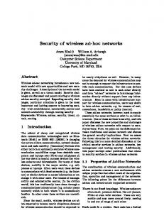
6 Discussion The results we have presented demonstrate that future ad hoc networks can scale well beyond the Gupta-Kumar capacity bounds attained when nodes simply try to avoid MAI [8]. First, we showed that the optimal capacity that any protocol architecture can attain in a wireless network   is Θ n2 r3 (n)/k . Second, we demonstrated that this capacity can indeed be attained when nodes embrace MAI as transmitters and receivers, and that a non-vanishing capacity is attainable per S-D pair even when information must be disseminated over multiple hops. Given that the majority of nodes in an ad hoc network are sources and destinations of information, we frame the rest of our discussion for the important case of k = Θ(n). The capacity under the SPR model when k = Θ(n) equals Θ(1/nr(n)), which is the well-known Gupta-Kumar result, and shows that avoiding MAI in the communication protocols of ad hoc networks does not scale. Given that today’s ad hoc networks are based on interference avoidance, it is clear that massively scalable ad hoc networks cannot exist without substantial changes to the way in which protocols are designed. 45 40

0.25

0.8 x n

35

2ηmin/(lkmax)

fRSP R = f × (1/(1 + κ))

The total number of transmitters in A is less than the total number of nodes in A. We have already shown that the total number of nodes is Θ(nr(n)). Under the MPTR model, each node can transmit a maximum of Θ(nr2 (n)) packets, and under the MPR model each packet trasnmits just a single packet. This provides the bounds for MPR and MPTR. To obtain the bound for SPR, we note that each transmitter silences all the nodes within an area of Θ(r2 (n)). Hence, only Θ(1/r(n)) nodes are capable of transmitting simultaneously across a cut. Each of these nodes transmits a single packet and, therefore, the above equation provides the bound for SPR. 

30 25 20 15 10

mean observed value minimum observed value maximum observed value

0.25

0.4 x n 5 0 0

2

4

n

6

8

10 6

x 10

Proof: (Sketch) Consider the Cut S in Figure 1. The capacity of this cut and hence the network is less than

Figure 4. Numerical results

(no. of transmitters in A) × (max. tranmission per node) (1/2)k (55)

On the other hand, under the MPR model [6] the network capacity is equal to Θ(r(n)), which constitutes a dramatic improvement over SPR, and promises to provide capacity

gains in practice by embracing interference at the receivers. However, to attain a non-vanishing capacity, r(n) must be Θ(1), i.e., use single-hop communication. Unfortunately, this is not feasible in practice, because of the energy that would be incurred in transmissions and the complexity required for the receivers to decode a number of transmissions in the order of the nodes in the network. In contrast to the above, MPTR achieves the optimal per-node capacity of Θ(nr3 (n)). Thus, any choice of r(n) = Ω(n−1/3 ) allows us to increase the per-node capacity of the network with n, while still having multihop communication. Moreover, the transmission range and hopsize decreases with n. As per our analysis, the capacity of a network is a constant factor of Γ, where Γ = 2ηmin /l(kmax ), such that ηmin is the minimum number of edges between any two squarelets, kmax is the maximum number of sources or destinations in a single squarelet and l × l is the total number of squarelets. To illustrate this, we numerically evaluated the behavior of Γ as a function of n. Figure 4 presents the mean, minimum and maximum observed value of Γ over a thousand network topologies randomly generated and in which k = n/2 and r(n) = 1/n0.25 . Clearly, as n → ∞ we have r(n) → 0. Nevertheless, the numerical results show that the per-node capacity still increases as Θ(n0.25 ). In closing, we should point out that, while our results provide a completely new outlook on the design of wireless ad hoc networks, much work remains to be done to fully understand their fundamental limits! For example, the results we have presented address only unicast traffic; our model can be used to study the cases of multicast and broadcast information dissemination. We also hope that this paper motivates research on protocol architectures that combine multi-packet reception and transmission to attain massively scalable ad hoc networks.

7 Acknowledgments This work was partially sponsored by the U.S. Army Research Office under grants W911NF-04-1-0224 and W911NF-05-1-0246, by the National Science Foundation under grant CCF-0729230, by the Defense Advanced Research Projects Agency through Air Force Research Laboratory Contract FA8750-07-C-0169, and by the Baskin Chair of Computer Engineering. The views and conclusions contained in this document are those of the authors and should not be interpreted as representing the official policies, either expressed or implied, of the U.S. Government.

References [1] R. Ahlswede, C. Ning, S.-Y. R. Li, and R. W. Yeung. Network information flow. IEEE Transactions on Information Theory, 46(4):1204–1216, 2000. [2] B. Bollabas. Modern Graph Theory. Springer Verlag, 1998.

[3] R. M. de Moraes, H. R. Sadjadpour, and J. J. Garcia-LunaAceves. Many-to-many communication: A new approach for collaboration in manets. In Proc. of IEEE INFOCOM 2007, Anchorage, Alaska, USA., May 6-12 2007. [4] L. R. Ford and D. R. Fulkerson. Flows in Networks. Princeton Univ. Press, 1962. [5] M. Franceschetti, O. Dousse, D. Tse, and P. Thiran. Closing the gap in the capacity of wireless networks via percolation theory. IEEE Transactions on Information Theory, 53(3):1009–1018, 2007. [6] J. J. Garcia-Luna-Aceves, H. R. Sadjadpour, and Z. Wang. Challenges: Towards truly scalable ad hoc networks. In Proc. of ACM MobiCom 2007, Montreal, Quebec, Canada, September 9-14 2007. [7] M. Grossglauser and D. Tse. Mobility increases the capacity of ad hoc wireless networks. IEEE/ACM Transactions on Networking, 10(4):477–486, 2002. [8] P. Gupta and P. R. Kumar. The capacity of wireless networks. IEEE Transactions on Information Theory, 46(2):388–404, 2000. [9] S. Katti, S. Gollakota, and D. Katabi. Embracing wireless interference: Analog network coding. In Proc. of ACM SIGCOMM 2007, Kyoto, Japan, August 27-31 2007. [10] P. Klein, S. A. Plotkin, and S. Rao. Excluded minors, network decomposition, and multicommodity flow. In Proc. of ACM symposium on Theory of computing, San Diego, California, USA, May 16-18 1993. [11] S. Kulkarni and P. Viswanath. A deterministic approach to throughput scaling wireless networks. IEEE Transactions on Information Theory, 50(6):1041–1049, 2004. [12] M. Kunde. Block gossiping on grids and tori: Deterministic sorting and routing match the bisection bound. In Proc. of European Symp. Algorithms, 1991. [13] P. Kyasanur and N. Vaidya. Capacity of multi-channel wireless networks: Impact of number of channels and interfaces. In Proc. of ACM MobiCom 2005, Cologne, Germany, August 28-September 2 2005. [14] T. Leighton and S. Rao. Multicommodity max-flow mincut theorems and their use in designing approximation algorithms. Journal of the ACM, 46(6):787–832, 1999. [15] J. Liu, D. Goeckel, and D. Towsley. Bounds on the gain of network coding and broadcasting in wireless networks. In Proc. of IEEE INFOCOM 2007, Anchorage, Alaska, USA., May 6-12 2007. [16] R. Madan, D. Shah, and O. Leveque. Product multicommodity flow in wireless networks. Submitted to IEEE Transactions on Information Theory, 2007. [17] A. Ozgur, O. Leveque, and D. Tse. Hierarchical cooperation achieves optimal capacity scaling in ad hoc networks. IEEE Transactions on Information Theory, 53(10):2549– 3572, 2007. [18] S. Toumpis and A. J. Goldsmith. Capacity regions for wireless ad hoc networks. IEEE Transactions on Wireless Communications, 2(4):736–748, 2003. [19] Y. Wu, P. A. Chou, and S.-Y. Kung. Information exchange in wireless networks with network coding and physical-layer broadcast. In Proc. of CISS 2005, Baltimore, MD, March 16-18 2005.