Optimal Scheduling in Sensor Networks Using Swarm Intelligence Kalyan Veeramachaneni and Lisa Ann Osadciw Department of Electrical Engineering and Computer Science Syracuse University, Syracuse, NY 13244-1240 Phone : 315 443 1319 Fax : 315 443 2583 kveerama,
[email protected] keywords:scheduling,swarm,evolutionary programming,sensor networks
Abstract - This paper presents a swarm intelligence based approach for optimal scheduling in sensor networks. Sensors are characterized by their transaction times and interdependencies. In the presence of interdependencies the problem of optimal scheduling to minimize the overall transaction/response time is modeled as a graph partitioning problem. Graph partitioning problem is a well known NPcomplete problem. A methodology and cost function is developed to solve the problem. A swarm intelligence based algorithm, particle swarm optimization (PSO) is used to solve the problem. The PSO algorithm solves the problem and emerges with a optimal schedule.
I. INTRODUCTION Multi sensor networks consist of varied sensor resources. Different mission requirements imply different sensors to be used at different times. When given a set of sensors for a particular mission, finding the optimal configuration of sensors as well as network parameters is a challenging problem. Scheduling the sensors in such a way that the total system transaction time or response time is reduced is another challenging problem. This paper presents a particle swarm optimization based approach to find the optimal sensor schedule in sensor networks. Each sensor is characterized by the time it needs for processing as well as communicating. Scheduling of these sensors is constrained by many practical issues such as communication concurrency constraints, interdependencies, and limited computational power at sink. The constraints limit the parallel operation of some of these sensors. These constraints are modeled as conflicts (for resources) between the sensors. In other words presence of a conflict between any two sensors would restrict parallel operation of those two sensors in the network. In the presence of such conflicts, the scheduling of these sensors and reducing the total processing time of the system is shown as an NP Complete problem. Scheduling, as presented in this paper, maximizes parallel operation in stead of sequentially following a schedule. An optimization problem is formulated for this solution. A memory-efficient evolutionary algorithm[3, 4, 5], particle
swarm optimization is used to solve this problem. The PSO generates the optimal schedule off-line, which is used by the sensor manager to schedule the sensors in real time. For example, the following two constraints are presented in the paper [1]: 1. Communication Concurrency Constraints: This constraint limits the sensors that can communicate or broadcast information simultaneously in a region. This problem has also been detailed previously in [2]. 2. Interdependencies: Certain Sensors are dependent on other sensors for carrying out their processing and hence cannot start until they are finished. In actual applications of sensor networks, there can be many more such constraints, which limit the parallel operation of two sensors. For example in a biometric sensor network, a camera can be used to take images of a face as well as any other physical attributes. The camera would be considered as two different sensors but have to take measurements one after another if the attributes are not in the same image. The face image may contain more than one usable image: face and iris. If the hand image is required, the camera needs to be used sequentially. Designing a schedule having the maximum parallelism reduces the total transaction time but may not minimize it. There are many alternative schedules with the same amount of parallelism achieving different values of total time. The constraints discussed above are used to design a compatibility graph
G c ( V, E ) for the N sensors in the system.
Each vertex in the graph represents a sensor. Presence of an edge indicates that those two sensors can be operated in parallel. In other words there are no constraints between these two sensors. Figure 1 shows a compatibility graph for 6 sensors for the conflicts given in equation (1).
C = { ( 1, 2 ), ( 1, 3 ), ( 1, 4 ), ( 1, 6 ), ( 4, 5, 6 ) } where
(1)
( S i, S j ..... S n ) are the sensors that have conflicts.
A conflicting graph can also be constructed based on the above data and is a complement of the compatibility graph.
This information in equation (1) is available to the sensor manager of the network and rarely changes over time. The subset of the sensors which have to be used depending upon the mission often changes as shown in [13].
cle, cost function, and the algorithm flowchart are presented in section 5. Section 6 presents the results achieved by using the PSO algorithm. Finally, Section 7 concludes the paper. II. MOTIVATION
1
Let the processing times for the 6 sensors be, as given, in Table 1. For convenience, the units of the time are left
2 6
3
unspecified and can be anything from µs to seconds. The conflicts and the corresponding compatibility graph are given in (1) and Figure 1. Once the maximum clique is found and the compatibility graph is partitioned, the following schedule can be obtained. Step 1: [1,5]
4
5
Fig. 1. Compatibility Graph for a set of 6 sensors for the conflicts presented in equation (1)
Now the optimal schedule can be determined by finding the maximum clique and partitioning the graph into cliques. A clique is a complete subgraph of the graph, where a complete graph is one such that each vertex pair is joined by an edge [6]. For example, in the above compatibility graph, (2,3,6) is a clique. “A graph is partitioned into cliques if its vertex set is partitioned into disjoint subsets, each one inducing a clique” [6]. A clique partitioning problem can be solved by iteratively searching the maximum clique of the graph and deleting it from the graph until there are no vertices left. For scheduling in the sensors networks, partitioning the compatibility graph into cliques and scheduling members of a clique together in a step (a time step) would reduce the total time of the system considerably by achieving maximum parallelism in sensors operation. However, with an increase in the number of sensors and hence the degree of the graph, the problem of finding the maximum clique becomes intractable. Graph partitioning algorithms only consider dividing the graph into maximum cliques. In sensor network application each node is a sensor and hence has its corresponding transaction time. Traditional graph partitioning algorithms would find the maximum clique in the graph, while this alone does not solve the problem in this case. In this application multiple maximum cliques are present in the graph and hence can be considered in finding the optimal schedule. In this paper a cost function is designed to evaluate the maximum cliques and hence select the optimal clique for the specific application. The evaluation is closely attached to the objective of the optimization, i.e., reducing the overall transaction time. In Section 2, a motivational example is presented. In Section 3, two additional concepts are presented and used to determine the value of a clique. Section 4 presents the particle swarm optimization algorithm. The design of each parti-
t s1 = max ( t 1, t 5 ) = 5units
TABLE 1. Processing times of sensors Sensor
Time (Units)
1
3
2
4
3
3
4
7
5
5
6
2
Step 2: [6, 3, 2] Step 3: [4]
t s2 = max ( t 2, t 3, t 6 ) = 4units
t s3 = max ( t 4 ) = 7units
Total processing time for the system is given by
t = t s1 + t s2 + t s3 = 16units It should be noted that the schedule presented above involved the maximum clique possible in the compatibility graph i.e., 2,3,6. The scheduler has hence scheduled them together. Alternatively, a different schedule can be Step 1: [1,5]
t s1 = max ( t 1, t 5 ) = 5units
Step 2: [4, 3, 2] Step 3: [6]
t s2 = max ( t 2, t 3, t 4 ) = 7units
t s3 = max ( t 6 ) = 2units
Total processing time for the system is given by
t = t s1 + t s2 + t s3 = 14units There is a considerable 12.5 % reduction in the total time of the system. Hence, this makes clear that clique partitioning the graph and finding maximum clique does not alone solve the problem. There are again many alternatives from which a selection has to be made. This also requires a search algorithm that will attempt to reduce the time as much as
possible. This paper presents an evolutionary algorithm and the methodology to solve this problem. III. OPTIMAL SCHEDULING AND GRAPH PARTITIONING In addition to the traditional graph partitioning algorithm, the key to optimal scheduling in sensor network application is the following 4 rules. 1. The clique with the maximum transaction time is given preference. The algorithm simultaneously tries to maximize the number of sensors running in parallel within the clique with the transaction time. After removing this clique from the graph, it iteratively repeats the procedure until all sensors are in a clique. 2. Always maximize the number of sensors in a clique. This reduces the total number of cliques after partitioning the whole graph. 3. A special weighting value is assigned to each clique to minimize the variation in sensor transaction time within the clique. The weight is defined as the average of the transaction times of the sensors in the clique. Besides minimizing the range of transaction values in the clique, this also saves only sensors with lower transaction times for further partitioning and reduces overall transaction time of the system. 4. Finally, a higher preference is given to the sensor with the most conflicts. This is because partitioning of such a sensor into a clique early on least affects the number of edges in the compatibility graph. It should be noted that the higher the number of edges in the compatibility graph, the greater the possibility of finding the optimal cliques is. These four rules result in values that are attached to the clique as it is formed and hence is evaluated in the algorithm for possible selection. Again these rules are specific to the application, i.e., reducing the overall transaction time of the system. These rules are incorporated as shown later in Section V. IV. PARTICLE SWARM OPTIMIZATION The particle swarm optimization algorithm, originally introduced in terms of social and cognitive behavior by Kennedy and Eberhart in 1995 [3], has come to be widely used as a problem solving method in engineering and computer science. PSO has since proven to be a powerful competitor to genetic algorithms [5]. The technique is fairly simple and comprehensible as it derives its simulation from the social behavior of individuals. The individuals, called particles, are flown through the multidimensional search space with each particle representing a possible solution to the multidimensional problem. The movement of the particles is influenced by two factors: its own best solution and any particle’s best solution. As a result of the first factor, its own best solution, each particle stores it in memory and experiences a pull towards this position, called pbest, as it
traverses through the search space. As a result of the second factor, the global best solution, the particle also stores this in memory and experiences a pull towards this position, called gbest. The first and the second factors are called cognitive and social components, respectively. After each iteration, the pbest and gbest are updated if a more dominating solution, in terms of fitness, is found by the particle and by the population, respectively. This process is continued iteratively until either the desired result is achieved or the computational power is exhausted. The PSO formulae define each particle in the D-dimensional space as X i = ( x i1, x i2, x i3 ..... x iD ) where the subscript i represents the particle number, and the second subscript is the dimension. The memory of the previous best position is represented as P i = ( p i1, p i2, p i3 ...... p iD ) , and a velocity along each dimension as V i = ( v i1, v i2, v i3 ..... v iD ) . After each iteration, the velocity term is updated, and the particle is pulled in the direction of its own best position, Pi, and the global best position, Pg, found so far. This is apparent in the velocity update equation, [12], (t + 1 )
V id
= ω × V id
(t )
(t)
+ rand ( 1 ) × Ψ 1 × ( p id – Xid ) + ( t)
rand ( 1 ) × Ψ 2 × ( p gd – Xid ) , and (t + 1) Xid
=
(t ) X id
+
(t + 1 ) V id .
(2) (3)
V. PROBLEM FORMULATION 1. Particle Representation The particle representation used in this paper is similar to the representation used by [7] for an individual in the genetic algorithm. Each particle has a dimension equal to the number of sensors ‘N’. Each particle has a binary representation and is a possible clique. For example ‘110011’ is a particle for 6 sensor systems and a ‘1’ implies presence of that particular sensor in the clique which the particle is representing. In the above example the clique contains Sensors 1,2,5,6. 2. The Cost Function The cost function is based on the two parameters presented in Section 3. Additionally a group weighting is also defined as elaborated below. C i = w1 × ( N ) + w 2 × ( T ) + w3 × ( W ) + w4 × ( C ) – p × ( N ) (4)
where N is number of sensors, ‘T’ is the transaction time of the clique, ‘W’ is the weight attached to this group of sensors. w 1 , w 2 , w3 , w 4 are the weights given to each one of them and w 2 >> w1 >> w 4 >> w 3 implying the importance of each one of them. The transaction time for a clique can be calculated as T = max ( t s ) i
(5)
where t si are the transaction times of the members (sensors) forming the clique. p =1000, if any of the dependencies are violated, (6) p =0, otherwise. A factor of “N” is multiplied to this value in the cost function. “N” is the number of sensors in that violate dependency in the clique. This gives proper direction to the swarm. In absence of this multiplication factor of “N”, higher the number of sensors in the clique higher will be value of the rest of the parameters added together. In successive iterations the swarm converges to a clique containing all the sensors considering that algorithm is based on maximization of cost function to achieve optimal results. The four parameters in the cost function are normalized. This normalization is done after merging the “pbest” and the “present” vectors together. After merging the whole new vector is normalized and then separated into respective pbest vector and present vectors. ‘W’ is the weight given to a clique. It is the average of the transaction times of the sensors forming the clique. This weight is necessary when there are two solutions each having equal number of sensors, and consisting the same dominating sensor in terms of transaction time. In such a case the first two ‘N’ and ‘T’ will be equal for both the cliques. However, a better solution will be the clique having the sensors with high transaction times when compared to other. For having this type of case covered the cost function has this additional value added defined as the weight given to the group. In [6] a greedy algorithm is presented to partition the graph into cliques. The algorithm does not however, partition the graph in minimum number of cliques which is optimum. It is not necessary that the optimum partitioning will always contain maximum cliques possible in the graph. It is observed that if a higher weight is given to the clique containing the node, which has highest number of conflicts or in this specific application the sensor with highest restriction in terms of operation, the iterative clique partition of the graph results in less number of cliques than the greedy approach. This is incorporated in the cost function as ‘C’. It is the summation of all the possible conflicts that the members of the clique have with the nodes still remaining in the graph to be partitioned. Intuitively, this makes sense since removal of that clique would not result in much loss of edges in the compatibility graph and leaves a lot of scope for further formation of cliques in remaining nodes. It can be seen from above discussion that the design of a cost function is very crucial for any optimization algorithm. For particle swarm optimization algorithm it gives the direction to the particles in the search space.
Load Transaction times Dependencies
Update Dependencies and Transaction Times
Output all the optimal groups/ cliques found by the PSO While
No
covering the whole graph
Sensors Still Left for Scheduling
Yes
Schedule one group after another
Call PSO and Pass Graph
Optimal Group of Sensors which form Clique
Save the Clique and Remove the sensors which formed the Optimal group
Fig. 2. Flowchart showing algorithm implementation
3. The Algorithm The particle representation is binary and hence binary PSO has been used to evolve the cliques. The dependencies and the transaction times are inputs to the PSO algorithm. The PSO finds the optimal maximum clique. The sensors forming this clique are removed and the dependencies are updated as well as the transaction times. The new dependencies and the transaction times are fed into the PSO again. This is repeated iteratively till all the sensors are grouped. The groups can now be scheduled one after another assuming that there is no specific sequence required. Figure 2 shows the flowchart of the algorithm implemented to find the optimal groups of the sensors, which can be run in parallel. The binary PSO as described in [12] is very similar to the continuous model in terms of velocity update as in (2). The
difference is in position update equations. The position update equation for the binary model is given by ifρ id < s ( v id ( t ) )thenx id ( t ) = 1 ;elsex id ( t ) = 0
(7)
1 s ( vid ) = --------------------------------1 + exp ( – v id )
(8)
7
3
1
8
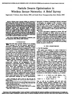
where ρ id is a vector of random numbers, drawn from a uniform distribution between [0,1]. VI. RESULTS AND DISCUSSION The algorithm has been applied to a set of 10 sensors. The transaction times and the dependencies are drawn at random. The transaction times for the sensors are given in Table II for both the data sets. Figure 3 is the compatibility graph for the first set of 10 sensors. In this graph each sensor is represented as a node. An edge between two nodes (sensors) imply that they can be operated in parallel. This compatibility graph is partitioned into cliques using the PSO. The resulting clique formation is shown in the graph and Table III. The overall transaction time is minimized and an optimal value of 62.1118 units is achieved for this data set. Alternatively, a greedy approach is applied to the graph and the resulting formation of cliques is presented in Table IV. The greedy approach tries to find the maximum clique possible in the graph, removes it from the graph, and iteratively does this till all the nodes in the graph are partitioned into cliques.
2
9
5
4
6
10
Fig. 3.Clique Partitioning of the Graph Using Particle Swarm Optimization TABLE III. OPTIMAL SCHEDULE FOR THE FIRST SET OF SENSORS Time Step
Sensors (PSO)
Transaction Times
Total Time
1
1, 2, 8
18.7367
18.7367
2
5, 6, 7
16.7738
35.5105
3
3, 4, 10
15.2140
50.7245
4
9
11.3873
62.1118
TABLE IV. OPTIMAL SENSOR SCHEDULE BASED ON GREEDY APPROACH TABLE II.TRANSACTION TIMES FOR THE TWO SETS OF DATA
Time Step
Sensors (Greedy)
Transaction Times
Total Time
Sensor #
Transaction Times: Data 1
Transaction Times: Data 2
1
1, 5, 6, 8, 10
14.3765
14.3765
Sensor 1
8.7556
7.6946
2
2, 4
18.7367
33.1132
Sensor 2
18.7367
1.5489
3
7
16.7738
49.8870
3
11.6713
61.5583
9
11.3873
72.9456
Sensor 3
11.6713
13.1263
4
Sensor 4
15.2140
16.7593
5
Sensor 5
5.8753
15.7698
Sensor 6
12.2965
11.8410
Sensor 7
16.7738
18.1799
Sensor 8
14.3765
4.6053
Sensor 9
11.3873
16.5234
Sensor 10
6.6304
17.6905
It should be noted that the algorithm can be modified to greedy approach by setting all other weights equal to zero except for w 1 and setting w 1 =1. A suboptimal result with transaction times 72.9456 units is achieved. Figure 4 is the conflict graph for the second set of data. Again each node represents the corresponding sensor. An edge between any two sensors, however, imply that they have a conflict and cannot be operated in parallel. It should be noted that conflict graph is a complement of the compatibility graph. A conflict graph is solved by the well known graph coloring technique. It does the same as the clique partitioning does to compatibility graph. By applying the PSO to the compatibility graph for the second set of data the cliques presented in Table V were achieved. In figure 4 the cliques are the nodes in same color. The overall transaction time is minimized to 54.1786 units.
VIII. REFERENCES
3 1
9
7
8
2
5 4
10
6
Fig. 4.Conflict Graph and Corresponding Optimal Graph Coloring Using PSO TABLE V.OPTIMAL SCHEDULE FOR SECOND SET OF SENSORS Time Step
Sensors (PSO)
Transaction Times
Total Time
1
3,7,9
18.1799
18.1799
2
5, 8, 10
17.6905
35.8704
3
1,4,6
16.7593
52.6297
4
2
1.5489
54.1786
[1]
Lloyd G. Greenwald, Harish Sethu, “On Scheduling Sensor Networks”, Proceedings of AAAI/KDD/UAI Joint Workshop on RealTime Decision Support and Diagnosis Systems, Edmonton, Alberta, Canada, July 29, 2002
[2]
Francesc Comellas, Javier Ozon, “Graph Coloring Algorithms for Assignment Problems in Radio Networks”, Applications of Neural Networks to Telecommunications, pp. 49-56, Lawerence Erlbaum Assoc. Inc. Pub., 1995.
[3]
Kennedy J. and Eberhart, R., “Particle Swarm Optimization”, IEEE International Conference on Neural Networks, 1995, Perth, Australia.
[4]
Eberhart R. and Kennedy J., “A New Optimizer Using Particles Swarm Theory”, Sixth International Symposium on Micro Machine and Human Science, 1995, Nayoga, Japan.
[5]
Eberhart R. and Shi Y., “Comparison between Genetic Algorithms and Particle Swarm Optimization”, The 7th Annual Conference on Evolutionary Programming, 1998, San Diego, USA.
[6]
Giovanni De Micheli, Synthesis and Optimization of Digital Circuits, McGraw Hill Inc. 1994.
[7]
Harpal Maini, Kishan Mehrotra, Chilukuri Mohan, Sanjay Ranka, “ Genetic Algorithms for Graph Partitioning and Incremental Graph Partitioning,
[8]
Shiyuan Jin, Ming Zhou, Annie S. Wu, “ Sensor Network Optimization Using a Genetic Algorithm”,
[9]
Kennedy J., “Small Worlds and MegaMinds: Effects of Neighbourhood Topology on Particle Swarm Performance”, Proceedings of the 1999 Congress of Evolutionary Computation, vol. 3, 1931-1938. IEEE Press.
[10]
Shi Y. H., Eberhart R. C., “Parameter Selection in Particle Swarm Optimization”, The 7th Annual Conference on Evolutionary Programming, San Diego, USA.
[11]
Carlisle A. and Dozier G.. “Adapting Particle Swarm Optimization to Dynamic Environments”, Proceedings of International Conference on Artificial Intelligence, Las Vegas, Nevada, USA, pp. 429-434, 2000.
[12]
Kennedy J., Eberhart R. C., and Shi, Y. H., Swarm Intelligence, Morgan Kaufmann Publishers, 2001.
[13]
Kalyan Veeramachaneni, Lisa Osadciw, Pramod Varshney, “ Adaptive Multimodal Biometric Fusion Algorithm Using Particle Swarm”, SPIE Aerosense, Orlando, Florida, April 21- 25, 2003.
VII. CONCLUSIONS This paper presented a graph partitioning based approach to group the sensors for parallel operation and scheduling. An evolutionary algorithm, particle swarm optimization algorithm has been used to search through space for an optimal solution. Traditionally, graph partitioning focusses on finding the minimum number of partitions of the graph. For minimizing transaction time for the sensor network scheduling application, it is shown that graph partitioning is not enough. Additional parameters have been added to the cost function to make a more robust design of the algorithm minimizing the transaction time. Alternative cliques are formed and evaluated by the algorithm while partitioning the graph and an optimal clique is selected. The algorithm has successfully found the optimal solutions leading to minimum overall transaction times for the system. Comparisons with the greedy graph partitioning algorithm show that better solutions can be found by applying constraints and costs to the clique formation. In future work, evolution of cost function weights specific to the input graph can be implemented using multiple PSO agents. Such algorithms show promise for better solutions.