research [22] â e.g. Branch-and-Bound [3] techniques â are being applied to prune ... how Branch-and-Bound techniques can be added to both the Promela ...
Optimal Scheduling using Branch and Bound with SPIN 4.0 Theo C. Ruys? Department of Computer Science, University of Twente. P.O. Box 217, 7500 AE Enschede, The Netherlands. http://www.cs.utwente.nl/~ruys/
Abstract. The use of model checkers to solve discrete optimisation problems is appealing. A model checker can first be used to verify that the model of the problem is correct. Subsequently, the same model can be used to find an optimal solution for the problem. This paper describes how the new Promela primitives of Spin 4.0 can be applied to search effectively for the optimal solution. We show how Branch-and-Bound techniques can be added to the LTL property that is used to find the solution. The LTL property is dynamically changed during the verification. We also show how the syntactical reordering of statements and/or processes in the Promela model can improve the search even further. The techniques are illustrated using two running examples: the Travelling Salesman Problem and a job-shop scheduling problem.
1
Introduction
Spin [10,11,12] is a model checker for the verification of distributed systems software. Spin is freely distributed, and often described as one of the most widely used verification systems. During the last decade, Spin has been successfully applied to trace logical design errors in distributed systems, such as operating systems, data communications protocols, switching systems, concurrent algorithms, railway signaling protocols, etc. [13]. This paper discusses how Spin can be applied effectively to solve discrete optimisation problems. Discrete optimisation problems are problems in which the decision variables assume discrete values from a specified set; when this set is set of integers, we have an integer programming problem. The combinatorial optimisation problems, on the other hand, are problems of choosing the best combination out of all possible combinations. Most combinatorial problems can be formulated as integer programs. In recent years, model checkers have been used to solve a number of nontrivial optimisation problems (esp. scheduling problems), reformulated in terms of reachability, i.e. as the (im)possibility to reach a state that improves on a given optimality criterion [2,5,7,8,15,20]. Techniques from the field of operations ?
This work is partially supported by the European Community IST-2001-35304 Project AMETIST (Advanced Methods for Timed Systems).
1
2
Theo C. Ruys
research [22] – e.g. Branch-and-Bound [3] techniques – are being applied to prune parts of the search tree that are guaranteed not to contain optimal solutions. Model checking algorithms have been extended with optimality criteria which provided a basis for the guided exploration of state spaces [2,15]. Though Spin has been used to solve optimisation problems (i.e. scheduling problems [5,20]), the procedures used were not very efficient and the state spaces were not pruned in any way. This paper shows how the new version of Spin can be used to effectively solve discrete optimisation problems, especially integer program problems. We show how Branch-and-Bound techniques can be added to both the Promela model and – even more effectively – to the property φ that is being verified with Spin. To improve efficiency we let the property φ dynamically change during the verification. We also show how the Promela model can be reordered syntactically to guide the exploration of the state space. The paper tries to retain the tutorial style of presentation of [18,19] to make the techniques easy to adopt by intermediate Spin users. The techniques are explained by means of running examples of two classes of optimisation problems. The effectiveness of the techniques are illustrated by some experiments. The paper is structured is as follows. In Section 2 we introduce the Travelling Salesman Problem and show how Spin can be used to find the optimal solution for this problem. Section 3 briefly describes the new primitives of Spin 4.0. In section 4 we show how the new primitives can be used to solve a TSP more effectively. In section 5 we apply the same techniques to a job-shop scheduling problems and show how Branch-and-Bound techniques can elegantly be isolated in the property which is being verified. The paper is concluded in Section 6. Experiments All verification experiments for this paper were run on a Dell Inspiron 4100 Laptop computer driven by a Pentium III Mobile/1Ghz with 384Mb of main memory. For all pan verification runs we limited the memory to 256Mb though. The experiments were carried out under Windows 2000 Professional and Cygwin 1.3.6; the pan verifiers were compiled using gcc version 2.95.3-5. For our experiments we used Spin version 4.0 (experimental, version: 8 Dec 2002). To compile the pan verifiers, we used the following options for gcc: GCC_SAFETY="-w -D_POSIX_SOURCE -DMEMLIM=256 -DSAFETY -DNOCLAIM -DXUSAFE -DNOFAIR" GCC_CLAIM="-w -D_POSIX_SOURCE -DMEMLIM=256 -DXUSAFE -DNOFAIR"
We executed the pan verifiers with the following directives: PAN_SAFETY="-m1000 -w20 -c1" PAN_CLAIM="-m1000 -w20 -a -c1"
The SAFETY-options relate to verifying safety properties and the CLAIM-options relate to verifying liveness properties (e.g. involving a LTL property).
2
TSP with plain Spin
The Traveling Salesman Problem (TSP) [16,17] is a well known optimisation problem from the area of operations research [22]. In a TSP, n points (cities) are given, and every pair of cities i and j is separated by a distance (or cost)
Optimal Scheduling using Branch & Bound with Spin 4.0
3
4
0
1
7 7
2
2
9 6
3
3
3
8
7
0 1 2 0 - 7 9 1 4 - 3 2 6 7 3 2 3 8
3 2 7 8 -
2
8
Fig. 1. Graph and matrix representation of the 4 × 4 example TSP.
cij . The problem is to connect the cities with the shortest closed tour, passing through each city exactly once. The TSP is NP-complete. A specific TSP can be specified by a distance (or cost) matrix. An entry cij in row i and column j specifies the cost of travelling from city i to city j. The entries could be the Euclidean distances between cities in a plane, or simply costs – making the problem non-Euclidean. Extensive research has been devoted to heuristics for the Euclidean TSP (see e.g. [17]). Construction heuristics for the non-Euclidean TSP are much less investigated. This paper considers non-Euclidean TSPs only. Modelling a TSP in Promela is straightforward. To illustrate the idea we develop a Promela model for the sample TSP of Fig. 1. Fig. 1 shows both a graph- and matrix-representation of a 4 × 4 TSP. The salesman itself is then modelled by a single process TSP. For each place i that the man has to visit, there is a label Pi in the process TSP. The salesman starts at label P0. From each label Pi the salesman can (non-deterministically) go to any label Pj that has not been visited yet. A bit-array visited is used to keep track of the places that have already been visited.1 If, after reaching place Pi, it turns out that all places have been visited, the salesman has to go back to place P0. To keep track of the travelling costs, a variable cost is used. This variable is initialised on 0. When we move from place Pi to Pj, this variable is updated with the cost cij from the cost-matrix of Fig. 1. Fig. 2 shows the Promela model of the TSP of Fig. 1. Now that we have a Promela model of the TSP, we want to use Spin to find the optimal route of the TSP. Fig. 3 shows a general procedure for finding an optimal solution for an optimisation problem using a model checker. The algorithm has been used in [5,20]. The algorithm iteratively verifies whether ‘the cost will eventually be greater than min’.2 Each time this property is violated, Spin has found a path leading to a final state for which the cost is less than min. For each error Spin generates an error trail which corresponds with the better route. As the number of possible routes is finite, at a certain point Spin will not find a route for which the cost is less than the min found so far. Consequently, 1
2
In this example we use Promela’s built-in support for bit-arrays. In our experiments, however, we used the bit-vector library as discussed in [18], as these bitvectors do not only occupy less space in the state vector, the manipulation of the vectors is also slightly faster. Note that the LTL property itself is translated to a never-claim in the Promela model.
4
Theo C. Ruys bit int
visited[3]; cost;
active proctype TSP() { P0: atomic { if :: !visited[1] -> cost = cost + 7 ; goto P1 :: !visited[2] -> cost = cost + 9 ; goto P2 :: !visited[3] -> cost = cost + 2 ; goto P3 fi ; } P1: atomic { visited[1] = 1; if :: !visited[2] -> cost = cost + 3 ; goto P2 :: !visited[3] -> cost = cost + 7 ; goto P3 :: else -> cost = cost + 4 ; goto end fi ; } P2: atomic { visited[2] = 1; if :: !visited[1] -> cost = cost + 7 ; goto P1 :: !visited[3] -> cost = cost + 8 ; goto P3 :: else -> cost = cost + 6 ; goto end fi ; } P3: atomic { visited[3] = 1; if :: !visited[1] -> cost = cost + 3 ; goto P1 :: !visited[2] -> cost = cost + 8 ; goto P2 :: else -> cost = cost + 2 ; goto end fi ; } end: }
Fig. 2. Promela model of a sample TSP with dimension 4.
the error trace which was generated last (corresponding with this optimal min) is the optimal route. This approach works, but is (highly) inefficient: the complete state space already contains the most optimal solution. After a single run over the state space one should be able to report on the optimal solution. The problem, however, is that we cannot compare information (e.g. the cost) obtained via different execution paths in standard Spin. This is inherent to the application of model checkers as a black box for solving optimisation problems.
3
Spin version 4.0
Spin version 4.0 [10] – available from [11] – supports the inclusion of embedded C code into Promela models through five new primitives: �
c decl: to introduce C types that can be used in the Promela model;
Optimal Scheduling using Branch & Bound with Spin 4.0
5
input: Promela model M with cost added to the states. output: the optimal solution min for the optimisation problem of M . 1 2 3 4 5 6
min ← (worst case) maximum cost do use Spin to check M � 3(cost > min) if (error found) then min ← cost while (error found)
Fig. 3. Algorithm to find the optimal solution for an optimisation problem using Spin. �
�
�
�
c state: to add new C variables to the Promela model. Such new variables can have three possible scopes: – global to the Promela model; – local to one of the processes in the model; or – hidden, which means that the variable will not end up in the state vector, but can be accessed in c expr or c code fragments. c expr: to evaluate a C expression whose return value can be used in the Promela model (e.g. as a guard); c code: to add arbitrary C code fragments as an atomic statement to the Promela model. For example, the c code primitive enables to include useful printf-statements in the verifier for debugging purposes. c track: to include (external) memory into the state vector.
The purpose of the new primitives is to provide support for automatic model extraction from C code. And although “it is not the intent of these extensions to be used in manually constructed models” [10], the extensions are helpful for storing and accessing global information of the verification process. Within c expr of c code fragments one can access the global and local variables of the currrent state through the global C variable now of type State. The global variables of the Promela model are fields in a State. For example, if the Promela model has a global variable cost, the value of this variable in the current state can be accessed using now.cost. As of version 4.0, the pan-verifier generated by Spin also contains a guided simulation mode. It is no longer needed to replay error trails with Spin. For more details on the new features of Spin 4.0 the reader is deferred to [10]. In the rest of this paper we will only use the primitives c state, c expr and c code.
4
TSP with Branch-and-Bound
In this section, we will discuss how the new C primitives of Spin 4.0 can be used to compute the optimal solution of a TSP more efficiently. We show how Spin
6
Theo C. Ruys
can be used to obtain the optimal solution in a single verification run. Branchand-Bound techniques can be used to prune the search tree. We also show how heuristics can be used to further improve the search.3 Spin 4.0 allows us to add hidden c state variables to the pan verifier within the Promela model. Consequently, while exploring the state space, each time Spin finds a better solution it can save this solution in such a hidden variable. To get the best route for our TSP problem with Spin 4.0, the TSP model has to be altered in the following ways: 1. Add a hidden, global variable best cost to the Promela model and consequently to the pan verifier. c_state "int best_cost" "Hidden" Due to the scope "Hidden", the variable best cost will not be stored in the state vector and will be global to all execution runs. 2. Initialise the variable best cost at the start of the verification – using a c code fragment – on MAX COST, where MAX COST is a worst-case estimate of the cost of a schedule: for all schedules the total cost will be lower than MAX COST. #define MAX_COST 1000 init { c_code { best_cost = MAX_COST; }; ... }
3. Whenever a new solution is found (i.e. when the label end is reached), the cost for that new route is compared with the best cost sofar. If cost is smaller, we have found a better solution, so the variable best cost is updated and the trace is saved: ... end: c_code { if (now.cost < best_cost) { best_cost = now.cost; printf("\n> best cost sofar: %d ", best_cost); putrail(); Nr_Trails--; } }
The function putrail saves the trace to the current state (i.e. it writes the states in the current DFS stack to a trail-file). The statement Nr Trails-makes sure that a subsequent call of putrail will overwrite a previous (less optimal) trail. 3
In this paper we only apply heuristics on the Promela level. Edelkamp et. al. [6] use a more powerful approach in HSF-Spin, where heuristics are applied in the internals of Spin.
Optimal Scheduling using Branch & Bound with Spin 4.0
7
Branch-and-Bound in the model. Branch-and-Bound [3,22] is an approach developed for solving discrete and combinatorial optimisation problems. The essence of the Branch-and-Bound approach is the following: – Enumerate all possible solutions and represent these solutions in an enumeration tree. The leaves are end-points of possible solutions and a path from the start node to a leaf represents a solution. – While building the tree (i.e. the state space), we can stop considering descendents of an interior node, if it is certain that all paths via this node will (i) either lead to an invalid solution or (ii) will have higher costs than the best path found so far. The Branch-and-Bound approach is not a heuristic or approximating procedure, but it is an exact, optimising procedure that finds an optimal solution. In our Promela model of the TSP problem, the Branch-and-Bound approach can be applied to ‘prune’ the state space. If in a place Pi the current cost is already higher than the best cost so far (i.e best cost), it is not useful to continue searching. So at the beginning of every place Pi of our model we add the following c expr: IF c_expr { now.cost > best_cost } -> goto end FI ;
Branch-and-Bound in the property. Recall the original idea of the algorithm of Fig. 3 which iteratively checks 3(cost > min) to find an optimal solution. Although inefficient, due to Spins on-the-fly model checking algorithm, for each subsequent iteration, less of the state space will be checked. For each execution path, Spin will stop searching as soon as it finds a state for which cost > min holds. Furthermore, Spin will exit with an error as soon as it finds an execution path for which the final cost is lower than min. So, in a way, Spin’s on-the-fly verification algorithm already performs some Branch-and-Bound functionality by default. Using the possibilities of Spin 4.0, we can improve the verification of the 3property by replacing min with the hidden global variable best cost. We define the following macro using a c expr statement: #define higher_cost (c_expr { now.cost >= best_cost })
and we check 3higher cost. In doing so – as the variable best cost is changed during the verification – the property that is being checked is dynamically changed during the verification! Nearest Neighbour Heuristic. When using Branch-and-Bound methods to solve TSPs with many cities, large amounts of computer time may be required. For this reason, heuristics, which quickly lead to a good (but not necessarily optimal) solution to a TSP, are often used. One of such heuristics is the “Nearest Neighbour Heuristic” (NN-heuristic) [22]. To apply the NN-heuristic, the salesman begins at any city and then visits the nearest city. Then the salesman goes to
8
Theo C. Ruys
1 2 3 4 5 6 7
procedure dfs(s: state) if error(s) then report error fi add s to Statespace foreach successor t of s do if t not in Statespace then dfs(t) fi od end dfs
Fig. 4. Basic depth-first search algorithm [14].
the unvisited city closest to the city it has most recently visited. The salesman continues in this fashion until a tour is obtained. In order to apply the NN-heuristic to Spin we must control the order in which neighbour places are selected. In order words, we must control the order of successor states in the state space exploration algorithm of Spin. The algorithm of Fig. 4 from [14] shows a basic depth-first search algorithm which generates and examines every global state that is reachable from a given initial state. Although Spin uses a slightly different (nested) depth-first search algorithm, for the discussion here, Fig 4 suffices. There is only one place in the algorithm where we can influence Spin’s depthfirst search: line 4, where the algorithm iterates over the successor states of state s. Spin always uses the same well-defined routine to order the list of successors. This list is ordered as follows: – Processes. Spin arranges the processes in reverse order of creation (i.e. stack order). That is, the process with the highest process id (pid) will be selected first. – Statements. Within each process, Spin considers all possible executable statements. For a statement without guards, there is at most one successor. For an if or a do statement, the list of possible successors is the (possible empty) list of executable guards in the same order as they appear in the Promela model. As the Promela processes can be created in any order and we are also free to order the guards within if and do clauses, we now have limited control over Spin’s search algorithm from within the Promela model. Fortunately, the control over the order of the guards within if-clauses is enough to apply the NN-heuristic to Spin. To make sure that in every place Pi, Spin will first consider the place Pj for which the cost cij is the lowest, the guards of all if-clauses are sorted on the cost cij , such that the guard with the lowest cost cij is at the top and the highest cost is at the bottom. Experimental results. To compare the different approaches w.r.t. the TSP, we have carried out some experiments with some randomly generated TSPs. The original approach which lets Spin iteratively check M � 3(cost > min) was left out of the experiments for obvious reasons. Table 1 lists the results of the
Optimal Scheduling using Branch & Bound with Spin 4.0
no B&B unsorted, B&B in model unsorted, B&B in property sorted, B&B in model sorted, B&B in property
9
dim = 11 dim = 12 dim = 13 dim = 14 dim = 15 572732 1878490 5459480 o.o.m. o.o.m. 278756 212987 514335 2478450 2820890 111922 72024 173311 1050580 1010080 132520 54927 140078 1748130 1388110 49803 16664 43242 737109 480574
Table 1. Verification results (number of states) of verifying Promela models of five randomly generated TSP cost matrices using different types of optimisation schemes.
experiments for randomly generated TSPs of dimension 11–15. We used a script to generate the cost-matrix for these TSPs where each cij was randomly chosen from the interval 1-100.4 We used another script to generate the Promela models for the particular TSP as described in this section. The entry ‘o.o.m’ stands for ‘out of memory’. For the Promela model without Branch-and-Bound functionality, not surprisingly, there is no difference between the cases where the guards of the ifclauses are either unsorted or sorted. Therefore we have only included one of them. From the experiments we can learn that the Branch-and-Bound in the property is more advantageous than the Branch-and-Bound in the model. This does not come as a suprise as due to the addition of Branch-and-Bound functionality in the Promela model, the number of states of the TSP process increases. It is also interesting to see that the NN-heuristic really pays of. As the cost matrices are randomly generated, we cannot compare the results for the different dimensions.
5
Personalisation Machine
In this section, we discuss the application of the Branch-and-Bound approach to a job-shop scheduling problem. We will extend the ‘Branch-and-Bound in the property’ technique as discussed in Section 4 by adding more bounding conditions to the property. Problem description. The problem itself is a simplified version of a case study proposed by Cybernetix (France) within the Advanced Methods for Timed Systems (AMETIST, IST-2001-35304) project [1]. Cybernetix is manufacturing machines for smart card personalisation. These machines take piles of blank smart cards as raw material, program them with personalised data, print them and test them. Fig. 5 shows a schematic overview of the personalisation machine that we discuss in this paper. Cards are transported by a Conveyer belt. There are NPERS Personalisation Stations where cards can be personalised. The conveyer 4
If the interval from which the different costs cij is (much) smaller, e.g. 1–10, the number of states will drop significantly due to Spin’s state matching.
10
Theo C. Ruys
�� ���� �� ��� ��� ��� ��� ��� ��� ��� ��� ��� �� �� �� ������ ������ ������ ���������� �� ������ ������ ���������� �� ������ ������� ��� � � � � � � ��� � � � � � � � � ������ ������ �������� �� ������ ������ �������� �� ������ ������ ��� ��� ����� ��� ������ �� ���� ����� Personalisation Stations
Unloading
Loading
Conveyer
Fig. 5. Schematic overview of the personalisation machine.
is NPERS+2 positions long. The Unloader puts empty cards on the belt. The Loader removes personalised cards from the belt. The order in which the cards are loaded from the belt should be same as the order in which they were unloaded onto the belt. The conveyer can only move a step to the right which takes tRIGHT time units. If cards are unloaded onto the belt or loaded from the belt, the conveyer cannot move. Unloading and loading can be done in parallel. Unloading and loading takes tUNLOAD resp. tLOAD time units. If after a conveyer move, an empty card is under a personalisation station, the card might be taken of the belt by the personalistion station and the personalisation of the card will start immediately. The personalisation of a card takes tPERSONALISE time units. In the original case study description, tRIGHT is equal to 1, tUNLOAD and LOAD are 2, whereas tPERSONALISE lies between 10 and 50. Goal. Given NPERS personalisation stations, the goal is to find an optimal schedule to personalise NCARDS cards. Promela model. Modelling the personalisation machine in Promela is straightforward. The conveyer belt is modelled by an array of NCELLS=NPERS+2 cells. A cell is represented by a short. If a cell has the value 0 it is empty. If a cell contains a value n>0 the cell contains an unpersonalised card with number n. If n i=NCELLS-1; do :: (i > 0) -> belt[i] = belt[i-1]; i=i-1 :: else -> break od; belt[0] = EMPTY; time = time + tRIGHT; } od }
The macro CARD ON BELT returns 1 if there is a card on the belt. The other two logical processes that ‘consume time’ are the Unloading and Loading process. Because unloading and loading might happen concurrently, the behaviour of both processes is modelled by a single process UnloaderLoader. The unloading part just puts cards on the belt. The loading part will remove cards from the belt and will check that the order of the cards is still correct. If not, it sets the time to -1. Below we only include fragments of the loading part of the UnloaderLoader process. If the last card has been taken from of the belt, we check whether the schedule found is faster than the best schedule so far. If this is the case, we update the hidden c state-variable best time. ::
atomic { (belt[LAST] == expectedCard) -> belt[LAST] = EMPTY; expectedCard = expectedCard-1; time = time + tLOAD; if :: ::
:: fi
expectedCard < -(NCARDS+1) -> assert(false) expectedCard == -(NCARDS+1) -> atomic { c_code { if (now.time < best_time) { best_time = now.time; Nr_Trails=0; putrail(); } }; break; } else
} ::
atomic { (belt[LAST] !=0 && belt[LAST] != expectedCard) -> time = -1; break; }
Each personalisation station is modelled by a process PersStation(i). When an unpersonalised card n is in belt[i], a personalisation station might start personalising this card n. Unlike the other processes, the process PersStation waits for time to pass. After it has taken an card from the belt it sets its finish time[i] to the time that it will have finished the personalisation of n (i.e. time + tPERSONALISE). Then the process starts waiting till the time has reached finish time[i].
12
Theo C. Ruys
Variable time advance. Because either the conveyer or unloader might have to wait for a personalisation station to finish, we also need a process which consumes ‘idle’ time. In our initial, naive model we used a process Tick which just increases the time by 1 time unit. The total number of ticks was bounded by a constant. The obvious disadvantage of this method is that the process Tick can always do a time tick; even when there are no personalisation stations currently ‘waiting’ for the time to reach their finishing time. Therefore, in our current model we follow Brinksma and Mader [5], who use the well-known variable time advance procedure [21]. With a variable time advance procedure, simulated time goes forward to the next moment in time at which some event triggers a state transition, and all intervening time is skipped. With respect to the personalisation machine this means that we let time jump to the finish time[i] > 0 which is the earliest. Heuristics. In the discussion on the algorithm of Fig. 4 we noted that we can guide Spin’s depth-first search by changing the order in which Spin considers successor states of a state s. Spin arranges the processes in reverse order of creation. That is, the process that is created last, will be selected first in considering the next successor state. For optimal schedules for the ‘personalisation machine’ it is clear that the number of idle time steps by the TimeAdvance process should be minimized. So a step of the TimeAdvance process should be the last step to be considered by Spin. Furthermore, as personalisation takes the longest time, starting the personalisation card should be considered first by Spin. Branch-and-Bound. Following the conclusions on the TSP, we want to apply the Branch-and-Bound approach using a dynamic bound in the property. We will check 3too late or wrong schedule, where the macro is defined as #define too_late_or_wrong_schedule \ (c_expr { (now.time >= best_time) || \ (now.time < 0) || \ (will_not_be_faster()) || \ (wrong_schedule()) \ })
The macro expands to a c expr expression which apart from the now familiar bound on the time and the test on negative time due to an incorrect schedule, containts two additional function calls: will not be faster and wrong schedule. These two functions try to decide at an early stage whether the current schedule leads to an inferior or incorrect schedule. Both C functions only use the current state (i.e. now) and the best time found so far. – The function will not be faster checks whether the minimum time to finish the cards that are still in the machine already exceeds the best time so far. The function only looks at the last card (i.e. the card with sequence number NCARDS) in the machine and computes the minimal time left for this card to reach the Loader.
Optimal Scheduling using Branch & Bound with Spin 4.0
13
– To signal incorrect schedules, the UnloaderLoader sets the time to -1 whenever a card is to be loaded from the belt which is out of order. It will be more advantageous, however, to discover such incorrect schedules (much) earlier. The function wrong schedule returns 1 if either one of the two conditions hold: �
�
Two personalised cards on the belt are out-of-order : ∃ 1 ≤ i, j ≤ NPERS + 1 : (i < j) ∧ (belt[i] < 0) ∧ (belt[j] < 0) ∧ (belt[i] < belt[j]) An personalised card is under a personalisation station containing a card with a lower original sequence number : ∃ 1 ≤ i ≤ NPERS : (belt[i] < 0) ∧ (−belt[i] > card in pers[i])
Both functions together are coded in less than 70 lines of C code. Get all optimal schedules. Due to the structure of the problem, Spin will always find just a single (optimal) schedule for a given time. The reason for this is that for all schedules with the same end-time, in the last-but-one state, the last card will be under the Loader. Due to state matching of Spin all these states will be regarded to be the same. To obtain all optimal schedules, an extra ‘magic number’ can be added to each state. The magic number ensures that each state will be unique. It is obvious that making the states unique will have a negative impact on the number of states. Experimental results. To compare the various optimisations on the model of the ‘personalisation machine’, we have carried out some experiments with several combinations of the Branch-and-Bound optimisations discussed. For these experiments we used the following values for the time-constants: tRIGHT=1, tUNLOAD=tLOAD=2 and tPERSONALISE=10. We have verified six different versions of the model. The models can be characterised as follows: v1 Model with a naive ordering of the creation of processes: UnloaderLoader, personalisation stations, Conveyer and finally TimeAdvance. The Branch-and-Bound functionality is isolated in the property, but we only bound on: “now.time >= best time || now.time < 0” v2 Model with an improved ordering of the processes: TimeAdvance, UnloaderLoader, Conveyer and finally the personalisation stations. Version v2 uses the same Branch-and-Bound approach as v1. v3 = v2, but adding “|| wrong schedule()” to the B&B property v4 = v2, but adding “|| will not be faster()” to the B&B property v5 = v2, but adding “|| wrong schedule() || will not be faster()” to the B&B property (so v5 = v3 + v4) v6 = v5, but adding a ‘magic number’ to each state (and thus obtaining all optimal schedules) Table 2 shows the results of verifying the different versions of the Promela model for different values of NPERS and NCARDS. It is clear that the optimisations
14
Theo C. Ruys
v1 v2 v3 v4 v5 v6
NPERS=3 NCARDS=4 states mem time 213760 23.1 4.5 161140 18.5 3.2 125501 12.1 2.4 9709