Optimal sensor location for overland flow network monitoring ... Therefore, monitoring in overland flow systems is a ... To the best of authors' knowledge, this approach has not been studied ..... The free-error approach (without sensor noises in ...
Optimal sensor location for overland flow network monitoring* Van Tri NGUYEN 1 , Didier GEORGES Abstract— The problem of optimal sensor location for monitoring of an overland flow network is addressed in this paper. The flow dynamics in each branch is described by the continuity equation of Saint-Venant model and Green-Ampt infiltration formula, while the initial states are assumed to be unknown. A methodology is then proposed to optimize the placement of sensors, with the purpose of estimating those states by a least square error minimization between measured and estimated water heights. Considering the method of variational calculus to solve for this minimization, a criterion based on the computed adjoint state is used to maximize the output sensitivity by appropriate sensor locations. A case-study of three small surface runoffs connected together at a point where two upper flows stream down into the third one is considered as an application example, and numerical simulations are provided with different measurement scenarios to validate the proposed optimal sensor location technique as well as the estimation method.
I. I NTRODUCTION Flood is a natural phenomenon that can cause a lot of effects on many aspects of human life. It happens when the water discharges of river, stream or drainage ditch exceed the maximum of its banks. The increment of water level on watercourse occurs under natural condition like a heavy rain, a rapid ice melting or human activities like a broken dam. In some special situations such as very excessive rainfall, hurricane or tropical storm, a flood can become a "flash flood" with duration less than six hours. It can be seen as a dangerous disaster with large destructive power, very high speed and unpredictability. Among the mechanism of flood, the extreme rainfall causing huge overland flow is a common one and not difficult to observe. Therefore, monitoring in overland flow systems is a key process to detect, predict and provide warning when there is a possibility of flood. The sensor network is necessary for observing the system of water flow. Because of technical and economic reasons, the number of sensors is limited. As a result, state estimation and reconstruction over the whole overland flow system from few measurements only should be achieved. Moreover, the sensor location and sensor number affect on the accuracy of estimation. An investigation of the optimal sensor placement is thus also needed before estimation step. In this work, an optimal sensor location for state estimation approaches based on adjoint analysis for an overland flow network is examined. The adjoint based state and parameters estimation method has been investigated by the authors in some former works ∗ This work has been partially supported by the LabEx PERSYVAL-Lab (ANR-11-LABX-0025-01) and the MEPIERA project, Grenoble INP 1 Univ. Grenoble Alpes, GIPSA-Lab, F-38000 Grenoble, France.
Email: {van-tri.nguyen, didier.georges, gildas.besancon}@gipsa-lab.grenoble-inp.fr
1
and Gildas BESANÇON
1
both with synthetic measurements [13], [15], [16] and real data [14]. These works have been realized on a single overland flow and the locations of sensor have been chosen manually. The adjoint method is used widely in both hydraulic and automatic researches in overland flow and open channel flow for identification (see [5], [6], [26] for details) and control (see [3], [7], [9] for details ). The discussion about these contributions can be seen in [13]–[16]. In the last four decades, the problem of sensor location determination has been addressed by various contributions. Bessousan [2], proposed the necessary and sufficient conditions for the existence of optimal sensor location by considering the sensor location as control variable of matrix Riccati equation; Amouroux et al. [1] and Omatu et al. [17] proposed optimal sensor position method for a fixed number of sensors by minimizing the trace of the error covariance matrix for a linear, timeinvariant system; Kumar et al. [10] studied also the infinitedimensional Riccati equation but using the minimization approach applied to a scalar measure of the error covariance matrix’s upper bound; Curtain et al. [4] proved that it exists an optimal location for finite sensors in linear distributed system and proposed a similar method to the work of Kumar et al. Other optimality criteria for sensor location are built on the observablity gramian for both linear and nonlinear systems. Muller et al. [11] used three criteria including the trace, the determinant and the minimum eigenvalue of the gramian inverse to find out the sensor location in a linear dynamical system; Waldraff et al. [24] and van den Berg et al. [23] added the condition number and the spectral norm of the gramian matrix as criteria; a nonlinear observability index has been used by Georges for optimal sensor and actuator locations [8] in nonlinear finite-dimensional system; Wouwer et al. [25] studied the determinant of the gramian matrix of nonlinear distributed process to optimally place the sensors for parameter estimation; Sing et al. [18] investigated the empirical observability gramian and measure for determining sensor placement. Some scalar functions based on the Fisher information matrix (FIM) have also been employed to determine the optimal location of sensor. Uci´nski et al. [20]–[22] investigated some criteria of FIM to determine the sensor trajectories in distributed systems; with the same measure, Tricaud et al. [19] applied the D-optimality (logdeterminant) of FIM to plan the trajectory of heterogeneous mobile sensors for parameter identification. In the present study, a new criterion based on adjoint gradient is proposed to find the appropriate locations of measurements positions which are used for state estimation in an overland flow network governed by nonlinear infinite-dimensional partial
differential equations (PDEs). The three above mentioned approaches (minimizing some criterion based on the error covariance matrix, using the observability gramian or the Fisher information matrix) demand a high computational complexity with the calculation of matrix size N 2 × N 2 (with N the state space dimension of the system) while the proposed approach requires only N × N matrix calculation. Moreover, the adjoint-based gradients used for estimation are employed as the criterion for sensor placement. There is no need to make any other calculations. This method allows, at the same time, to measure the impact of the sensor positions on the performance of estimation algorithm. To the best of authors’ knowledge, this approach has not been studied before. The rest of this paper is structured as follows. The system dynamics and the formulation of optimal state estimation and sensor location are given in section II. Section III discusses about the adjoint analysis for state estimation. The criterion for optimally choosing sensor locations is described in section IV. A numerical implementation to illustrate the effectiveness of established method is included in section V. Finally, conclusion of paper is stated in section VI. II. S YSTEM DYNAMIC , OPTIMAL STATE ESTIMATION AND OPTIMAL SENSOR LOCATION
A. System dynamics The overland flow network considered hereafter is made of three small runoffs taking place on three spatial domains called Ω1 = [a1 , a3 ], Ω2 = [a2 , a3 ] and Ω1 = [a3 , a4 ] with spatial variables (x1 , x2 , x3 ) ∈ Ω1 × Ω2 × Ω3 . The interconnection point is at position a3 where two upstream flows called system 1 (denoted Σ1 ) and 2 (denoted Σ2 ) run into the downstream flow called system 3 (denoted Σ3 ) as shown in Fig. 1. a1 Σ1 Σ3 a3
a4
Σ2 a2
= infiltration rate on system Σn , (m/s); S0n = bed slope, (m/m); The initial and boundary conditions of system 1 and ( 2 are given by Dirichlet( conditions as follows. h1 (x1 , 0) = hi01 (x1 ) h2 (x2 , 0) = hi02 (x2 ) Σ1 Σ2 h1 (a1 , t) = hb01 (t) h2 (a2 , t) = hb02 (t) For the system 3, the initial condition is h3 (x3 , 0) = hi03 (x3 ). The confluence condition of water flow per width unit of three system at position a3 is specified by equation (2) f3 (a3 , t) = f1 (a3 , t) + f2 (a3 , t) (2) The boundary state of system 3 is specified by the depth of upstream flows. Initial conditions of all the systems hi01 (x1 ), hi02 (x2 ) and hi03 (x3 ) are unknown and need to be estimated. B. Optimal state estimation formulation and optimal sensor location The optimal state estimation proposed in this paper can be considered as an optimization problem where the desired initial state of all three systems are obtained from the minimization of the output measurement error in the least square sense. The observations together with the initial value (of optimization) are the inputs of the estimation algorithm and have impact on the algorithm estimation accuracy. Let us consider a cost function called J defined as a double integral in space and time of a measurement function. There are many ways to choose this function such as the sum of the squared discrepancies between the measured and simulated flow height on a time interval, or the sum of the absolute errors or the maximum of errors [12]. In this study, under the assumption of having sensor over all the three flows without any loss of generality, the cost function is defined by equation (3). The sensor locations denoted by x1j1 , x2j2 and x3j3 , respectively for systems 1, 2 and 3, will be optimally chosen by solving optimal sensor location problem described hereafter. Because of the lack of space, the notation h(x, t) will be reduced to h and the notation I(n) = {3, 3, 4} with n = {1, 2, 3} used with meaning I(n) = 3 if n = 1, I(n) = 3 if n = 2 and I(n) = 4 if n = 3. ( M ZT ( aZI(n) 3 n X 1X 4(xn −xnjn )hn dxn J= 2 j =0 n=1 n an 0 (3) ) ) 2
Fig. 1: Overland flow network configuration. Each overland flow system is governed by a PDE of flow height as described in equation (1). This is the continuity equation of the Saint-Venant model (see [15] for more details). ∂hn (xn , t) ∂fn (hn (xn , t)) + = rn (xn , t) − in (xn , t) ∂t ∂xn (1) n = {1, 2, 3} for Σ1 , Σ2 and Σ3 where xn = position on system Σn , (m); t = time, (s); hn (xn , t) = water flow depth of system Σn , (m); 5/3 1/2 fn (hn (xn , t)) = hn S0n /ηn = flow per width unit of 2 system Σn , (m /s) with the Manning roughness coefficient ηn ; rn = variable rainfall rate on system Σn , (m/s); in
−hmeas (xnjn , t) n
dt
where T = optimization horizon (hours); M1 , M2 and M3 = number of flow depth observation values in system 1, 2, 3 respectively; hmeas (x1j1 , t)= measured flow depth at the flow 1 depth observation position x1j1 of system 1 where x1j1 ∈ [a1 , a3 ] and j1 ∈ [0, M1 ]; the same meaning for the notations hmeas (x2j2 , t) and hmeas (x3j3 , t). The term 4(xn − xnjn ) 3 2 is an approximation of Delta-Dirac function described by a 2 2 Gaussian function 4(xn −xnjn ) = e−(x−xnjn ) /σ /Λ(xnjn ) with a very small variance σ 2 centering at position xnjn and aI(n) R 2 2 Λ(xnjn ) = e−(xn −xnjn ) /σ dxn . an
III. A DJOINT METHOD FOR STATE ESTIMATION The optimization issue for optimally finding the initial state of systems is to minimize the cost function J . The system dynamics given by equation (1) are equality constraints of the minimization problem. The continuity of first partial derivatives of both cost function and system equations allows to use the Lagrangian method to deal with equality constraints. Let us consider the objective functional L, defined on the functional space L2 ([a1 , a3 ], [0, T ]) × L2 ([a2 , a3 ], [0, T ]) × L2 ([a3 , a4 ], [0, T ]) × L2 ([a1 , a3 ]) × L2 ([a2 , a3 ])×L2 ([a3 , a4 ]) into R with three Lagrangian multipliers λ1 (x1 , t), λ2 (x2 , t) and λ3 (x3 , t), as the following equation. ) (ZT aZI(n) 3 X λn (xn , t)Σn dxn dt L=J + n=1
0
an
The optimal values of initial states can be found at the point where the first variation of cost functional with respect to estimating variables vanish for all values of the variation vector π = [δh1 (x1 , t) δh2 (x2 , t) δh3 (x3 , t) δhi01 (x1 ) δhi02 (x2 ) δhi03 (x3 )]. Firstly, the first variation of L is evaluated by considering two parts, J and the 3 remaining terms called K. The variation of cost function J is given as, " aZI(n) ( M ZT aZI(n) 3 n X X 4(xn −xnjn ) δJ = 4(xn − xnjn ) n=1
jn =1 0
an
an
# ×hn dxn −
hmeas (xnjn , t) n
)
δhn dxn dt
(4) and also the first variation of K is obtained by using integration by part technique: ( aZI(n)" # T ZT aZI(n) 3 X ∂λn δhn dxn dt δK = λn δhn dxn − ∂t n=1
0
an
0
an
aI(n) # ) ZT " ZT aZI(n) ∂fn ∂fn ∂λn + λn δhn dt − δhn dxn dt ∂hn ∂hn ∂xn an
0
0
an
(5) The first variation or the Gâteaux derivative of L in direction of vector π can be written under from of an inner product of π and the weak form of gradient of L, denoted ∇L as δL =< ∇L, π > where ( ZT aZI(n) 3 X < ∇L, π >= ∇Lhn δhn dxn dt n=1 aI(n)
Z + an
0
an
∇Lhi0n (xn ) δhi0n (xn )dxn
) (6)
The vector of weak form gradient ∇L has 6 elements ∇L = [∇Lh1 ∇Lh2 ∇Lh3 ∇Lhi01 (x1 ) Lhi02 (x2 ) Lhi03 (x3 ) ]. According to the first order necessary condition for optimality, the gradient ∇L must be equal to
zero to cancel the variation in all possible directions or ∇L = 0 (7) Each element of ∇L can be formulated by collecting the terms relating its corresponding variation in equations (4) and (5) (for instance δh1 for ∇Lh1 , δhi01 (x1 ) for ∇Lhi01 (x1 ) ) and compare the found formulation with the definition of inner product in equation (6). By applying the optimality condition (7) on the weak gradients for three system variables h1 , h2 and h3 one can obtained the adjoint systems of λ1 (x1 , t), λ2 (x2 , t) and λ3 (x3 , t) being dual to the direct ones, are governed by the PDEs given in equation (8). " aZI(n) Mn ∂λn ∂fn ∂λn X 4(xn −xnjn ) − + 4(xn −xnjn ) − ∂t ∂hn ∂xn j =0 n an # × hn (xn , t)dxn − hmeas (xnjn , t) = 0 with n = {1, 2, 3} n (8) The weak gradients of L with respect to the initial states are the terms multiplied with δhn (xn , 0) where n ∈ {1, 2, 3} under the spatial integral. The optimal estimation initial state will be determined such that these gradients are equal to zero through an appropriate algorithm. ∇Lhi0n (xn ) = −λn (xn , 0) with n = {1, 2, 3} (9) According to the necessary conditions for optimality, the goal is to force the first variation of the objective functional to zero. The remaining terms of equations (4) and (5) (after gradients formulation) are collected together and set to zero to find the initial and boundary conditions for the adjoint systems. ( aZI(n) 3 X − λn (xn , T )δhn (xn , T )dxn n=1
an
aI(n)) # ZT " ∂fn + λn δhn dt = 0 ∂hn 0
an
Because all the boundary conditions of the 3 systems are already fixed, their variations are equal to zero, δh1 (a1 , t) = 0, δh2 (a2 , t) = 0. To render the variations of δh1 (x1 , T ), δh2 (x2 , T ), δh3 (x3 , T ) and δh3 (a4 , t) equal to zero, the following initial conditions are set for the adjoint systems: λ1 (x1 , T ) = 0, λ2 (x2 , T ) = 0, λ3 (x3 , T ) = 0 and λ3 (a4 , t) = 0. The last time integrals are gathered as follows: ZT h ∂f1 ∂f2 λ1 (a3 , t) (a3 , t)δh1 (a3 , t) + λ2 (a3 , t) (a3 , t) ∂h1 ∂h2 0 i ∂f3 × δh2 (a3 , t) − λ3 (a3 , t) (a3 , t)δh3 (a3 , t) dt = 0 (10) ∂h3 The variation of the interconnected condition at position a3 , the interconnection point, is given by δf3 (a3 , t) = δf1 (a3 , t) + δf2 (a3 , t). By inserting this equation into (10) and removing the time integral, the following equalities are obtained: λ1 (a3 , t) = λ3 (a3 , t) and λ2 (a3 , t) = λ3 (a3 , t) These boundary conditions of the three adjoint systems reflect the confluence condition (2) of the direct ones.
From the previous analysis, the gradients in equation (9) represent the sensitivity of objective functional with respect to the initial conditions. The best observability will be obtained with the greatest sensitivity represented by absolute value of the gradients. The value of adjoint variable λn (xn , t) depends directly on the measurements which also depend on the observation position. As a result, the quality of estimation result depends on adjoint gradients with respect to the sensor position or combination of positions if several sensors are used. The optimal sensor positions will be the result of an optimization problem defined as the maximization of an index function of the gradients. A natural idea is to maximize the absolute minimal value of gradients. This means that the selected locations will guarantee the observability of all the initial states distributed over the domains. By denoting the combination of discretized observation positions selected as ξ and the set of all the position locations on the three domains Ω1 , Ω2 and Ω3 as χ = {xi1 , xj2 , xk3 } where 0 < i ≤ N1 − 1 with 4x1 = (a3 − a1 )/N1 , 0 < j ≤ N2 − 1 with 4x2 = (a3 − a2 )/N2 and 0 < k ≤ N3 − 1 with 4x3 = (a4 − a3 )/N3 , the optimization problem needing to be solved to find optimal sensor locations is formulated as follows:� T max min [abs (−λ1 (x1i ) , −λ2 (x2j ) , −λ3 (x3k ))] ξ∈χ
(11) The set {xi1 , xj2 , xk3 } is the discretized position of the sensor location domain {x1j1 , x2j2 , x3j3 } in equation (3). The minimization of the gradient absolute values in equation (11) is called as index function. One of the important factor in this optimization issue is the number of sensor being used. In this work, the placement of at most 3 sensors is considered. The number of combinations exponentially increase with a large number of sensors. As a result, some adequate integer programming approaches should be used to overcome the combinational issue. For a given number of sensors, all possible combinations of sensor locations over the domain Ω1 ×Ω2 ×Ω3 is first calculated. The minimum of sensitivity function is then evaluated for each combination. The optimal sensor position is finally found by checking the maximum of these minima. V. N UMERICAL IMPLEMENTATION Because of the non-linearity and complexity of direct and adjoint system equations, they can not be solved analytically. For that reason, they are discretized and solved numerically by using Lax-Wendroff finite-difference scheme (see [16] for details). As a result, the continuous gradients in equation (9) are evaluated at each points on discretized spatial domain of each flow, x1i , x2j and x3k . These gradients are used as inputs of the optimization algorithm which is based on the f mincon function of M atlab. The Broyden-FletcherGoldfarb-Shanno (BFGS) method is chosen to update the Hessian matrix. The free-error approach (without sensor
noises in the simulations) is used for evaluation procedure. This means that the synthetic measurements at the chosen locations are obtained from a system simulation with desired values of the initial conditions. The numerical implementation is realized on three overland flows chosen with different characteristics for the sake of illustration. The initial conditions for initial state estimates are the same for both sensor placement and state estimation and are chosen around the "real" ones. A. Optimal sensor location The approach presented in section IV for sensor location is illustrated here for three cases corresponding to three different numbers of available sensors: 1, 2 or 3. Each system is divided into 10 sections with 11 discrete positions, and the location problem is considered to be limited to possible locations at "interior positions". Obviously at the interconnection point, the final positions of system 1 and system 2 are physically the same, and identical to the first point of system 3. As a result, a total of 28 discretized points all over the flow network will be taken into account. (1) Case of 1 sensor: there are here exactly 28 possible positions for the sensor location, called "position combinations". Fig. 2 depicts the distribution of index function in equation (11) over all those possible discrete position combinations. One can see that the sensor must be located at combination number 28, which corresponds to the discrete position 10 of system 3. Notice that in the figure, index values above 10−3 also highlight some candidates which can still be of interest, such as position 2 on system 3 which gives the index value 0.0017. (2) Case of 2 sensors: here each −3
7
x 10
Index function with different positions of 1 sensor Index function
6
5
Index function
IV. O PTIMAL SENSOR LOCATION
4
3
2
1
0
5
10
15
20
25
Combination
Fig. 2: Index function with different location of 1 sensor. sensor can be placed wherever on the three systems, giving rise to 378 possible combinations, Fig. 3 shows that their optimal solution corresponds to combination 357, with index function value 0.0071 and it corresponds to discrete positions {3, 10} on system 3. The next sub-optimal combination is {8, 10} on system 3 with index function value 0.0066. (3) Case of 3 sensors: in this case one has 3276 position
Case Sensor number 1 2 3 4 5 6 7
1 1 2 2 3 3 3
Combination
Index function value
{10} on Ω3 {2} on Ω3 {3, 10} on Ω3 × Ω3 {8, 10} on Ω3 × Ω3 {10, 3, 10} on Ω1 × Ω3 × Ω3 {3, 3, 10} on Ω1 × Ω3 × Ω3 {4, 5, 10} on Ω3 × Ω3 × Ω3
0.0062 0.0017 0.0071 0.0066 0.0109 0.0103 0.0098
Estimation relative error System 1 System 2 System 3 17.20 % 24.60 % 2.33 % 20.45 % 93.20 % 36.37 % 10.20 % 18.14 % 0.81 % 15.78 % 21.88% 2.04 % 0.10 % 1.04 % 0.09 % 10.78% 19.46 % 0.52 % 10.55 % 20.72 % 1.5 %
TABLE I: The table of estimation error with different sensor numbers for three systems. −3
x 10
Index function with different combinations of 2 sensors
8
Index function 7
Index function
6
5
4
3
2
index function 0.0098. One can observe that at least 1 sensor must be placed at the end of system 3 This result seems to be reasonable because the last positions of system 3 contains more information propagated from the upstream systems and also the downstream one. The positions of other sensors depend on the physical characteristics of the system and initial values used for initial conditions in the algorithms, while each initial profile corresponds to a specified sensor configuration. In order to make the proposed approach more robust to initial conditions, the idea can be to run it for a large number of situations, and consider the average optimal result. This will be more deeply studied in our future work.
1
B. Optimal state estimation
0 50
100
150
200
250
300
350
Combination Estimation of initial state of system 2 0.22
0.2
0.18
Initial state
Fig. 3: Index function with different location of 2 sensors. combinations with time to evaluate the index function for all combinations is approximately 3505 second (on a PC Intel(R) Core(TM)2 Duo CPU P8600 @2.40 GHz, 3Go RAM with Matlab R2011b 32 bit). As shown in Fig. 4, the best sensitivity for state estimation is obtained here with combination 2286 at the end of Fig. 4, maximizing the value of index function at 0.0109. This corresponds to positions {10, 3, 10} on Ω1 × Ω3 × Ω3 . According to Fig. 4, there are
0.16
0.14
Estimated value Index function with different combinations of 3 sensors
Real value
0.12
0.012
Initial value Index function 0.1 20
0.01
60
80
100
120
140
160
180
x (cm)
Fig. 5: Estimation of initial state of system 2.
0.008
Index function
40
0.006
0.004
0.002
0 500
1000
1500
2000
2500
3000
Combination
Fig. 4: Index function with different location of 3 sensors. also other combinations which give reasonable sub-optimal solutions such as: {3, 3, 10} (on Ω1 ×Ω3 ×Ω3 ) corresponding to combination 655 and index function 0.0103 and {4, 5, 10} (on Ω3 × Ω3 × Ω3 ) corresponding to combination 3246 and
The estimation process is realized with 7 cases according to the number of sensors. Table I summarizes the considered combinations of sensors with the corresponding estimation relative errors and index function values. It can be seen that when 1 sensor is used and located at position 10 on Ω3 , a good estimation of initial state of system 3, while some errors remain for the upstream systems. The same situation occurs with case 2 when the sensor is located at position {2} also on Ω3 . The relative errors in this case are yet larger than in case 1 due to its index function value lower than the first one. The remaining errors in both cases may be due to mismatches between numerical methods used for sensor placement and state estimation, and will be investigated further in future works. When the number of sensors is increased to 2, as in cases 3 and 4, the estimation accuracy
also increases for all the systems. Once can for instance see that the combination {3, 10}, giving more sensitivity, allows to get smaller estimation errors. Four cases of 3 sensors are then examined. In case 5, two sensors are placed on system 3 and one sensor is at the end of system 1. The estimation of initial states of the system 1 converge with pretty small relative errors. Fig. 5 shows the estimation result of case 5 (for system 2 only due to space limitation). With a larger index function value, the sensor locations in this case provide more sensitivity for estimation than the last two cases. Moreover, one can observe that in cases 6 and 7, the estimation errors are close to the one of case 3. This means that the sensor positions {3, 4} on Ω1 seem not to bring significant additional information. From the above analysis, the presented optimal sensor placements gives an effective criterion to choose appropriate locations of sensor which allow the estimation algorithm to achieve good accuracy for the given initial conditions. VI. C ONCLUSION The issue of optimally locating a given number of sensors for state estimation in an overland flow network was addressed. In the proposed approach, the state estimation is formulated as a minimization problem of a cost function based on measurements, and the classical Lagrangian multiplier method is used to deal with the system dynamics. The calculus of variations is then applied on the Lagrangian functional in order to get the gradients, which are used not only as inputs of optimization process but also as a criterion to optimally locate the sensors. Some first results are presented and discussed with a numerical example: the optimal locations for 1, 2 or 3 sensor are firstly found for a given initial condition. The optimization process for state estimation is then performed with the computed optimal locations and compared to results obtained with some non optimal locations to assess the effectiveness of the proposed approach. Because from the estimation of initial condition one can recover the whole transient state by simulation, the method presented in this paper can be applied to determine the optimal location for some other hyperbolic systems like channel flows, traffic system flows to monitor the system. A deeper robustness analysis of the approach will be part of future works, as well as an extension to the case of optimal sensor location for both state and parameter estimation. R EFERENCES [1] M Amouroux, JP Babary, and C Malandrakis. Optimal location of sensors for linear stochastic distributed parameter systems. In Distributed Parameter Systems: Modelling and Identification, pages 92–113. Springer, 1978. [2] Alain Bensoussan. Optimization of sensors’ location in a distributed filtering problem. In Stability of stochastic dynamical systems, pages 62–84. Springer, 1972. [3] Tehuan Chen, Zhigang Ren, Chao Xu, and Ryan Loxton. Optimal boundary control for water hammer suppression in fluid transmission pipelines. Computers & Mathematics with Applications, 69(4):275– 290, 2015. [4] Ruth F Curtain and Akira Ichikawa. Optimal location of sensors for filtering for distributed systems. Springer, 1978.
[5] Yan Ding, Yafei Jia, and Sam S Y Wang. Identification of Manning’s Roughness Coefficients in Shallow Water Flows. Journal of Hydraulic Engineering, 130(6):501–510, June 2004. [6] Yan Ding and Sam S. Y. Wang. Identification of Manning’s roughness coefficients in channel network using adjoint analysis. International Journal of Computational Fluid Dynamics, 19(1):3–13, January 2005. [7] Yan Ding and Sam S.Y. Wang. Optimal control of flood diversion in watershed using nonlinear optimization. Advances in Water Resources, 44:30 – 48, 2012. [8] Didier Georges. The use of observability and controllability gramians or functions for optimal sensor and actuator location in finitedimensional systems. In Decision and Control, 1995., Proceedings of the 34th IEEE Conference on, volume 4, pages 3319–3324, New Orleans, LA, 1995. IEEE. [9] Didier Georges. Infinite-dimensional nonlinear predictive control design for open-channel hydraulic systems. Networks and Heterogeneous Media, 4(2):267–285, June 2009. [10] Sudarshan Kumar and John H Seinfeld. Optimal location of measurements for distributed parameter estimation. Automatic Control, IEEE Transactions on, 23(4):690–698, 1978. [11] PC Müller and HI Weber. Analysis and optimization of certain qualities of controllability and observability for linear dynamical systems. Automatica, 8(3):237–246, 1972. [12] TH Nguyen and DJ Fenton. Identification of roughness in open channels. In Proc. of 6th International Conference on Hydro-Science and Engineering, Brisbane, Australia, 2004. [13] Van Tri Nguyen, D. Georges, and Gildas Besançon. Adjoint-methodbased estimation of manning roughness coefficient in an overland flow model. In American Control Conference (ACC), 2015, pages 1977– 1982, Chicago, United States, July 2015. [14] Van Tri Nguyen, D. Georges, Gildas Besançon, and I. Zin. Application of adjoint method for estimating manning-strickler coefficient in Tondi Kiboro catchment. In Control Applications (CCA), 2015 IEEE Conference on, pages 551–556, Sydney, Australia, Sept 2015. [15] Van Tri Nguyen, Didier Georges, and Gildas Besançon. Optimal state estimation in an overland flow model using the adjoint method. In Control Applications (CCA), 2014 IEEE Conference on, pages 2034– 2039, Antibes/Nice, France, 2014. IEEE. [16] Van Tri Nguyen, Didier Georges, and Gildas Besançon. State and parameter estimation in 1-d hyperbolic {PDEs} based on an adjoint method. Automatica, 67:185 – 191, 2016. [17] Sigeru Omatu, Satoru Koide, and Takasi Soeda. Optimal sensor location problem for a linear distributed parameter system. Automatic Control, IEEE Transactions on, 23(4):665–673, 1978. [18] Abhay K Singh and Juergen Hahn. Optimal sensor location for nonlinear dynamic systems via empirical gramians. In Proceedings DYCOPS, volume 7, Boston, Massachusetts, 2004. [19] Christophe Tricaud, Maciej Patan, Dariusz Uci´nski, and YangQuan Chen. D-optimal trajectory design of heterogeneous mobile sensors for parameter estimation of distributed systems. In American Control Conference, 2008, pages 663–668, Seattle, WA, 2008. IEEE. [20] Dariusz Uci´nski. Measurement optimization for parameter estimation in distributed systems. Technical University Press Zielona Góra, 1999. [21] Dariusz Ucinski. Optimal sensor location for parameter estimation of distributed processes. International Journal of Control, 73(13):1235– 1248, 2000. [22] Dariusz Uci´nski and Maciej Patan. D-optimal design of a monitoring network for parameter estimation of distributed systems. Journal of Global Optimization, 39(2):291–322, 2007. [23] FWJ Van den Berg, HCJ Hoefsloot, HFM Boelens, and AK Smilde. Selection of optimal sensor position in a tubular reactor using robust degree of observability criteria. Chemical Engineering Science, 55(4):827–837, 2000. [24] Walter Waldraff, Denis Dochain, Sylvie Bourrel, and Alphonse Magnus. On the use of observability measures for sensor location in tubular reactor. Journal of Process Control, 8(5):497–505, 1998. [25] Alain Vande Wouwer, Nicolas Point, Stephanie Porteman, and Marcel Remy. An approach to the selection of optimal sensor locations in distributed parameter systems. Journal of process control, 10(4):291– 300, 2000. [26] Wenhuan Yu. A Quasi-Newton Method for Estimating the Parameter in a Nonlinear Hyperbolic System. Journal of Mathematical Analysis and Applications, 231(2):397–424, March 1999.