Expert Systems with Applications PERGAMON
Expert Systems with Applications 18 (2000) 257–269 www.elsevier.com/locate/eswa
Optimal signal multi-resolution by genetic algorithms to support artificial neural networks for exchange-rate forecasting Taeksoo Shin, Ingoo Han* Graduate School of Management, Korea Advanced Institute of Science and Technology, 207-43 Cheongryangri-Dong, Dongdaemoon-Gu, Seoul 130-012, South Korea
Abstract Detecting the features of significant patterns from historical data is crucial for good performance in time-series forecasting. Wavelet analysis, which processes information effectively at different scales, can be very useful for feature detection from complex and chaotic time series. In particular, the specific local properties of wavelets can be useful in describing the signals with discontinuous or fractal structure in financial markets. It also allows the removal of noise-dependent high frequencies, while conserving the signal bearing high frequency terms of the signal. However, one of the most critical issues to be solved in the application of the wavelet analysis is to choose the correct wavelet thresholding parameters. If the threshold is small or too large, the wavelet thresholding parameters will tend to overfit or underfit the data. The threshold has so far been selected arbitrarily or by a few statistical criteria. This study proposes an integrated thresholding design of the optimal or near-optimal wavelet transformation by genetic algorithms (GAs) to represent a significant signal most suitable in artificial neural network models. This approach is applied to Korean won/US dollar exchange-rate forecasting. The experimental results show that this integrated approach using GAs has better performance than the other three wavelet thresholding algorithms (cross-validation, best basis selection and best level tree). 䉷 2000 Elsevier Science Ltd. All rights reserved. Keywords: Artificial neural networks; Foreign-exchange rate markets; Chaos analysis; Genetic algorithms; Hill-climbing algorithms; Wavelet transform
1. Introduction Detecting the features of significant patterns from historical data is crucial for getting good performance in timeseries forecasting. The methods used for time-series analyses are conventionally based on the concepts of stationarity and linearity. Linear models such as autoregressive (AR), moving average (MA) and mixed (ARMA) models are often used under the conventional concepts. However, for cases in which the system dynamics are highly nonlinear, the performance of traditional models might be very poor. Artificial neural networks (ANNs) have demonstrated great potential for time-series forecasting. Lapedes and Farber (1987) first proposed using multi-layer feedforward neural networks for nonlinear signal prediction. Since then, research using (ANNs) has justified their use for nonlinear time-series forecasting. Recently, there has been a renewal of interest in linear expansions of signals, particularly using wavelets and some * Corresponding author. Tel.: ⫹ 82-2-958-3613; fax: ⫹ 82-2-958-3604. E-mail addresses:
[email protected] (T. Shin), ighan@kgsm. kaist.ac.kr (I. Han).
of their generalizations (Daubechies, 1992; Mallat, 1989; Rioul & Vetterli, 1991). Wavelet theory provides a mathematical tool for hierarchically decomposing signals and, hence, an elegant technique for representing signals at multiple levels of detail. A new data-filtering method (or multi-signal decomposition) namely, wavelet analysis is considered useful in comparison to other methods for handling the time series that contain strong quasi-cyclical components. Wavelet analysis theoretically presents much more clear local information according to multi-resolution learning. The multi-resolution framework in wavelet theory is employed for decomposing a signal and approximating it at different levels of detail. Unlike traditional neural network learning processes, multi-resolution learning exploits the approximation sequence representation-byrepresentation from the coarsest to the finest version during the neural network training process. Liang and Page (1997) showed that multi-resolution learning significantly improves the generalization ability of neural networks and, therefore, their effectiveness on difficult signal prediction problems. Generally the multi-signal decomposition method— Fourier analysis and wavelet analysis—is a good method
0957-4174/00/$ - see front matter 䉷 2000 Elsevier Science Ltd. All rights reserved. PII: S0957-417 4(00)00008-7
258
Taeksoo Shin, Ingoo Han / Expert Systems with Applications 18 (2000) 257–269
for the extraction of cyclical information-bearing signals from corrupted observations. In particular, the wavelet method having this advantage is considered a concept that needs to be developed further for use in short-term financial and economic time series showing chaotic temporal patterns. To date, the financial market studies related to wavelet analysis are increasingly being applied to many different applications (Aussem, Compbell & Murtagh, 1998; Cody, 1994; Greenblatt, 1996; Høg, 1996, 1997; McCabe & Weigend, 1996; Pancham, 1994; Tak, 1995). The principal objective of this paper is to develop a new hybrid system of optimal signal multi-resolution representation to support ANNs for foreign-exchange rate (FX) forecasting. In this study, the multi-scale signal representation of Neural networks (NNs) is supported by a wavelet transform (WT) as the multi-signal decomposition technique to detect the features of significant patterns. We apply the model architecture to forecasting the Korean won/US dollar returns in the FX market one day ahead of time. A strategy is devised using WT to construct a filter that is significantly matched to the frequency of the time series within the combined model. This study uses a backpropagation neural network model (BPN Rumelhart, Hinton & Williams, 1986) as a basic timeseries forecasting model. However, the conventional ANN building needs lengthy experimentation, which is a major roadblock in the extensive use of the method. Recently, it has been suggested that a few combined-model architectures using several algorithms improve performance. Our study includes this combined-model architecture. Through experimental results with wavelet filtering techniques, this paper also demonstrates various filtering criteria of wavelet analysis to support the NN learning optimization. Then, we analyze critical issues concerning optimal or near-optimal filter design problems in wavelet analysis, including the human expert as model developer confronted with the subjective problem of finding the optimal filter parameter to generate significant input variables for the forecasting model. Finally, we suggest a new near-optimal filtering criterion of multi-signal decomposition methods from our experimental learning and validation results of the NNs. That is, we propose a new extended NN that consists of a fourlayered architecture having a multi-scale extraction layer before arriving at the input layer. The model learning is supported by genetic algorithms (GAs) and a hill-climbing algorithm (HC). Through their hybrid learning, we tried to solve the present threshold problems in the optimal filter design efficiently while extracting significant information from the original data. The rest of this paper is organized as follows. In the next section, we briefly review the multi-resolution approach of financial markets. Then, multi-resolution techniques to WT are introduced. Section 4 suggests a new methodology for the hybrid system using GAs. The experimental results are in Section 5. The final section contains concluding remarks.
2. Multi-resolution approach to financial markets 2.1. Fractal structure of chaotic foreign-exchange rate markets An exposure to foreign-exchange risk could affect a firms investment decisions and, hence, distort the optimal allocation of resources. Therefore, knowledge acquisition of the temporal properties of foreign currency rates can have important implications for these issues. Recently, NNs as forecasting models for FXs have been investigated in a number of studies (Kuan & Liu, 1995; Refenes, 1993; Weigend, Rumelhart & Huberman, 1991; Weigend, Huberman & Rumelhart, 1992; Wu, 1995; Zhang & Hu, 1998). Fractional Brownian Motion (fBm) has long been considered a plausible model for financial markets, including the FX market. A fractal structure of the financial market, indicating the presence of correlations across time, hints at the possibility of forecasting. The recent advances in time– frequency localized transforms by applied mathematics and electrical engineering communities also provide us with new methods for the fBm process. In fact, it has been proven by Wornell (1990, 1993) that the WT with a Daubechies basis is an optimal transform for the fBm process. The structure of the financial market also has the feature of market heterogeneity. Market heterogeneity suggests that the different intentions among market participants result in sensitivity by the market to several different time scales. Different types of traders view the market with different time resolutions, for example, hourly, daily, weekly and so on. Short-term traders evaluate the market at high frequency and have a short memory. Small movements in the exchange rate mean a great deal to the short-term trader. Long-term traders evaluate lower frequency data with a much longer memory of the past data. They are only interested in large movements in the price. These different types of traders create the multi-scale dynamics of the time series. The above two features of the financial market reinforce the fact that multi-resolution embedding using wavelet analysis is very useful for discovering whether some time scales are more predictable than others. For example, one of the WT applications is to determine if the fractal dimension of a market indicator maintains consistency through different levels of scale. The reason is that the selection of the orthonormal wavelet used in the transform may influence the results, since these wavelets are themselves recursively defined and fractal in nature. To most closely reflect the heterogeneous structure of financial markets on our forecasting model, we use an ANN and wavelet analysis as our forecasting tools in this study. 2.2. Multi-resolution analysis using wavelet transforms The investigation of multi-scale representations of signals and the development of multi-scale algorithms has been a
Taeksoo Shin, Ingoo Han / Expert Systems with Applications 18 (2000) 257–269
Fig. 1. Two-dimensional (time–frequency) resolution of: (a) a short-term (or windowed) Fourier transform (Young, 1993); and (b) discrete wavelet transform (Young, 1993).
topic of interest in many engineering fields. In some cases such as the use of fractal models for signals, the motivation has directly been the fact that the phenomenon of interest exhibits important patterns through multi-scales. The second motivation has been the possibility of developing highly parallel and iterative algorithms based on such representations. The wavelet analysis is a robust tool that may be used to obtain qualitative information for highly nonstationary time series. Specifically, it may be used to detect a small-amplitude harmonic forcing term even when the dynamics are chaotic and for short total times (Permann & Hamiltion, 1992). Each stage of resolution can be considered a space that could represent a linear combination of some suitable basis. Each resolution space is a subset of a resolution space with a higher resolution. We intuitively view high-frequency noise differently from broad, low-frequency components due to, for example, baseline effects. By employing the multi-resolution view, we can build and dismantle curves according to the resolution level, so the wavelet functions are constructed to focus on different resolution details in the signal at different positions. This feature is possible because of the special structure of the wavelet basis functions. Fig. 1(a) shows the time–frequency resolution cells for the short-term Fourier transfrom (STFT) or the windowed Fourier transform (WFT). The window size controls the shape of these rectangles but the rectangles will be identical everywhere across the plane. So the resolution does not
259
change. For the Fourier case, as the frequency increases, the number of cycles of the exponential within the window increases whereas the number of cycles in every element is identical for the wavelet elements. Thus, for WTs, the “image” of the mother wavelet looks identical at every scale and translation; the image is either dilated or compressed to create the scaled version. Fig. 1(b) displays an important property of WTs. Their property includes that at high frequencies the time windows are very narrow, providing good time localization but poor frequency localization since the WT still has to obey the Heisenberg uncertainty principle (Masters, 1995). At low frequencies, the time windows are wide (longer in time) while the frequency windows are narrow. These windows are particularly useful since most natural signals exhibit long low-frequency features and short high-frequency features. This implies inherent support for multi-resolution analysis, which correlates with time series that exhibit self-similar behavior across different time scales. It allows simultaneous decomposition of a time series into components or basis functions that are localized in both time and frequency. The wavelet analysis procedure consists of the adoption of a wavelet function called the mother wavelet. The mother wavelet dictates the properties (efficiency, resolution, redundancy, noise immunity, etc.) of the wavelet decomposition. The STFT has its own limitations compared to the WT. For example, the discrete Fourier transform (DFT) spreads frequency information over all time and so there is a loss of frequency characteristics of time series in the time domain. The DFT process is said to be nonlocal in the time domain. We can partially compensate for this lack of localization by applying the STFT to introduce time dependency. But, the STFT filters, where time–frequency resolution cell (TFRC) has equal dimensions, are evenly spaced in the frequency domain (Fig. 1(a)). On the other hand, the dimension of the TFRCs in the WT changes along the frequency axis (Fig. 1(b)). For low frequencies, the windows are wide in time and narrow in frequency, giving good frequency resolution. For high frequency, the windows are wide in frequency and narrow in time, allowing good time resolution. Such a covering of the time-frequency plane is sometimes referred to as constant-Q analysis and is very effective for signal analysis (Rioul & Vetterli, 1991). The Q stands for the quality factor of a digital filter, i.e. the ratio between bandwidth and center frequency. The discrete WT (DWT) filter is related to a scaling function equal to two (Fig. 1(b)). The scaling function could be any number, even a fraction. In addition, the filter bandwidths in the STFT are constant while the DWT filters are, again, related by a factor of two. Thus, for DWT filters, the width of the filter is proportional to its center frequency. One way of looking at this is that the wavelet approach partitions the data into blocks of equal information content, representing a potentially useful characteristic of wavelet filters. Fig. 2 shows an example of multi-resolution of a DWT filter using daily Korean won/US dollar returns. The DWT filter is defined as Daubechies
260
Taeksoo Shin, Ingoo Han / Expert Systems with Applications 18 (2000) 257–269
Fig. 2. An example of the (a) daily Korean Won/US Dollar Returns; and (b) two-dimensional (time–frequency) resolution of a discrete wavelet transform (Daubechies wavelet with four coefficients).
wavelet with four coefficients (DAUB4; Press, Teukolsky & Flannery, 1992) in our study.
approximations at each level m of resolution are treated to yield the approximation and the detail coefficient obtained at the next level m ⫹ 1: But, the applications of the transform to both the detail and the approximation coefficients result in an expansion of the structure of the tree algorithm to the full binary tree (Coifman & Wickerhauser, 1993). This is called a wavelet packet transform (WPT). It is a more general transform than the DWT. The main difference is that, while in the DWT the detail coefficients are kept and the approximation coefficients are further analyzed at each step, in the WPT both the approximation signal and the detail signal are analyzed at each step. This results in redundant information, as each level of the transform retains n samples. Therefore, the WPT produces an arbitrary frequency split, which can be adapted to the signal. While wavelet packets create arbitrary binary slicing of frequencies (with associated time resolution), they do not change over time. Often, a signal is first arbitrarily segmented and then the wavelet packet decomposition is performed on each segment in an independent manner. There exist simple and efficient multi-resolution algorithms for both the DWT and the WPT. They select the most efficient basis out of the given set of bases to represent a given signal. In the most efficient basis, some of the coefficients attain high values while the remaining ones show low values. The respective basis vectors represent relevant information. 3.2. Highpass, lowpass and bandpass filters
3. Multi-resolution techniques to wavelet transforms There are several ways to look at the WT. This section presents major characteristics of the WT and introduces multi-resolution techniques to WTs. 3.1. Discrete wavelet transform and wavelet packet transform The DWT is expressed as a pyramid or tree algorithm (Mallat, 1989). In the pyramid algorithm the detailed branches are not used for further calculations and only the
The subspaces created by the WT roughly correspond to the frequency subbands partitioning the frequency bandwidth of the data set. These subspaces then form a disjointed cover of the frequency space of the original data set. In other words, the subspaces have no elements in common and the union of the frequency subbands spans the frequency span of the original data set. Any set of subspaces, which are a disjointed cover of the original data set, is understood on an orthonormal basis. The WT basis is, then, but one of a family of orthonormal bases with different subband intervals. According to the
Fig. 3. The four basic filter types by frequency-response characteristics.
Taeksoo Shin, Ingoo Han / Expert Systems with Applications 18 (2000) 257–269
Fig. 4. Proposed research framework.
frequency-response characteristics, the frequency subbands or subspaces are again categorized into the four basic filter types, i.e. lowpass, highpass, bandpass and bandstop filters as shown in Fig. 3. Lowpass filters allow all frequencies below the specified frequency to pass and are usually employed for smoothing. Highpass filters allow all frequencies above the specified frequency to pass. They are usually used to extract information on local variation while suppressing overall signal levels. Bandpass filters allow only those periodic components in the vicinity of the specified frequency to pass. Bandstop filters behave exactly opposite to bandpass filters. The most basic type of filter from which practically all other filters are derived is the bandpass filter. As the name implies, this filter passes a single band of periodic components, stopping all components having higher or lower frequencies. The lowpass, highpass and bandpass filters used in this study are characterized by two parameters, i.e. frequency and width. The center frequency is the frequency maximally favored by the filter. It may be any value from 0.0 to 0.5 (the Nyquist frequency) cycles per sample. The reciprocal of the frequency parameter is exactly the period of the periodic component. The width defines the width of the passband. The passband indicates the band of frequency components that are allowed to pass. The width is specified in the same units as the frequency, and it typically ranges from approximately 0.01 to 0.2. The width-parameter is difficult to specify. There is no simple calculation to provide the correct value. It is an arbitrary choice. Unfortunately, a real tradeoff is involved. It is essentially related to the Heisenberg uncertainty principle (Masters, 1995). 3.3. The optimal multi-resolution techniques of time series using wavelet transforms The multi-resolution analysis framework in wavelet
261
theory is employed for decomposing a signal and approximating it at different levels of details. Unlike traditional NN learning, which employs a single signal representation for the entire training process, multi-resolution learning exploits the approximation sequence representation-byrepresentation from the coarsest to the finest version during the NN training process. Since the analysis process is iterative, in theory it can continue indefinitely. In reality, the multi-resolution or decomposition can proceed only until the individual details consist of a single sample. In practice, a suitable number of levels will be selected based on the nature of the signal or a suitable criterion such as entropy. There are a few optimal multi-resolution techniques in previous studies: (1) the best basis selection (Chen, 1995; Chen & Donoho, 1995; Chen, Donoho & Saunders, 1998; Coifman & Wickerhauser, 1992; Daubechies, 1988; Donoho, 1995; Mallat & Zhang, 1993); (2) the crossvalidation (Jensen & Bultheel, 1997; Nason, 1994, 1996); and (3) the best level tree (Coifman, Meyer, Quake & Wickerhauser, 1994). An additivity-type property of WT is well suited for efficient searching of binary-tree structures and the fundamentals of splitting. Classical entropy-based criteria match these conditions and describe information-related properties for an accurate representation of a given signal. Entropy is a common concept in many fields, mainly in signal processing while these criteria have a few limitations in choosing the optimal decomposition subseries from original time series. That is, they have problems such as inefficient learning and mis-specification of a fitness function for global model optimization. Therefore, we suggest a new criterion of choosing the optimal decomposed subseries from original series by DWTs to solve these problems in the following research model architecture.
4. Research design and experiments 4.1. A hybrid neural network model architecture In general, for an one-dimensional discrete-time signal, the high frequencies influence the details of the filter levels while the low frequencies influence the deepest levels and the associated approximations. The original signal can be expressed as an additive combination of the wavelet coefficients at the different resolution levels. In this section, we suggest our research framework and develop a new hybrid NN architecture as shown in Figs. 4 and 5. Our research framework consists of four phases. The first phase decomposes the financial time series into different decomposed series components using a DWT. In the second phase, we extract the refined highpass, lowpass and bandpass filters from the decomposed time series that are based on the feedback from the next phase. Fig. 5 shows our hybrid NN as extended NN architecture in comparison to prior models. We extract a significant scale component
262
Taeksoo Shin, Ingoo Han / Expert Systems with Applications 18 (2000) 257–269
Fig. 5. A hybrid neural network model architecture.
generation automatically from the original data within our model. This function achieves a multi-scale extraction layer of our model. The third phase uses a neurogenetic approach to learn NNs with GAs and then the fifth phase includes an additional weight learning process by HC to reinforce a generalization of learning parameters or weights generated in the previous phase. For this purpose, the fourth phase is compared with the third phase in terms of the forecasting accuracy. The resolution of time series can be adjusted to local parameters to detect its present features including promising features in close time areas with more sensitivity. Using multiple scales of resolution, the time-series forecasting can be refined in the areas. Feature-based segmentation techniques detect local features such as transitions, lines and curves, in general referred to as edges, based on the values of appropriate local operators. To improve local prediction, the signal parameters such as the refined lowpass, highpass and bandpass filters are proposed to control multiple scales of resolution within our research framework. For example, when our time series is decomposed into 10 scales, each scale is then multiplied by a weighting factor (0–1) and then the weighted transform is inverted back to a new meaningful time series. In summary, our hybrid model efficiently extracts the significant temporal information from the original data by the globally optimal filter design using a hybrid NN and GA. The reason is as described below. Among the various cost measures that one can choose for finding adaptive time–frequency decompositions, we select evolutionary data-driven criteria using GA. There are two major benefits. Our model architecture uses the final performance measure of the BPN model within a unified model framework as fitness function for the optimal wavelet thresholding. Eq. (1) represents the fitness function to lead to the correct solution of our hybrid BPN. This function solves the mixed optimization problem. It includes optimiz-
ing simultaneously both the multi-resolution or wavelet thresholding cut-off parameters as parts of learning parameters and the other learning parameters of the BPN. It also solves the generalization problems of our hybrid model. 1 0v uN uX Min@t
yi ⫺ y^i 2 =N A
1 i1
y^i f
IWTi ; IWTi
l2 X
BANDi
j;
jl1
HP
l1 ; l2 ; BP
l1 ; l2 ; LP
l1 ; l2 僆 IWTi ; s:t: Xi
k X
BANDi
j; 1 ⱕ l1 ⱕ l2 ⱕ k
j1
where yi actual output of the i case of population at
t ⫹ 1 day, y^i NN output model of the i case of population at
t ⫹ 1 day, f
· NN model, IWTi the i case of refined wavelet filtered inputs of population at (t) day, Xi the i input case of population at (t) day, BANDi
j the j automatically decomposed time series by Daubechies wavelet transform (DAUB4) of the i case of population at (t) day, HP(l 1,l 2) highpass filtered inputs, BP(l 1,l 2) bandpass filtered inputs, LP(l 1,l 2) lowpass filtered inputs, N the population size, l the time-lag index, k the maximum length of decomposition levels of pyramid or tree algorithms,
Taeksoo Shin, Ingoo Han / Expert Systems with Applications 18 (2000) 257–269 Table 1 Frequency and energy (power) corresponding to decomposed band series of daily Korean won/US dollar returns
ln Xt ⫺ ln Xt⫺1 Decomposed band series
Frequency
Energy (power)
Band Band Band Band Band Band Band Band Band Band
1025–2048 513–1024 257–512 129–256 65–128 33–64 17–32 9–16 5–8 1–4
762.362905 272.263314 65.286306 37.198682 16.772893 6.330478 2.911817 2.363013 1.593836 0.916059
1 2 3 4 5 6 7 8 9 10
l1 lL1 ; the cut-off frequency (or scale) level for the lowpass filter on condition of
l2 lL2 k; l2 lH2 ; the cut-off frequency level for the highpass filter on condition of
l1 lH1 1 except that both l 1 and l 2 are l B1 and l B2, the cut-off frequency levels for the bandpass filter on condition of
1 ⱕ l1 ⱕ l2 ⱕ k: 4.2. Phase I: decomposing the daily exchange rate time series using discrete wavelet transform The first step of the proposed search framework shown in Fig. 4 is to decompose the daily exchange rate using DAUB4. The decomposition of a time series into hidden cycles using the DWT is based on the scalogram analysis of the time series with respect to a fixed wavelet basis (Arino & Vidakovic, 1995). The scalogram (Rioul & Flandrin, 1992) is defined as a wavelet periodogram referring to the absolute value of the wavelet coefficients at each scale. The scalogram is usually plotted logarithmically as a function of both the scale and location indices. The inspection of the scalogram (or of the wavelet coefficients themselves) is useful when one needs to view frequency/scale and location information at the same time. In the same manner that the periodogram produces an ANOVA decomposition of energy of a signal to different Fourier frequencies, the scalogram decomposes the energy to level components (see Table 1). Thus, the scalogram of the DWT of a time series is the key tool used to decompose the series into cycles of different
263
frequencies as decomposed band series. However, it is not a trivial task for model experts to extract the hidden cyclic structure from the original data by analyzing the distribution shape of the scalogram as shown in Fig. 6. Fig. 7 shows the pyramid or tree algorithm (Mallat, 1989) applied to the daily Korean won/US dollar returns to generate decomposed band series from the time series. We can extract a lowpass filter, highpass filter and bandpass filter from the decomposed band series (i.e. Bands 1–10) in the figure. For example, Band 1 corresponds to the highest frequency component in the data. This band component indicates signals with very short periods. In addition, we can effectively extract a bandpass filter to the data by eliminating the highest and lowest bands from the total bands. Therefore, we combine some of the decomposed band series (Bands 1–10) by the DWT into generating separately three refined lowpass, highpass and bandpass filters as the optimally refined wavelet filters defined in the following phase. 4.3. Phase II: extracting the refined wavelet filters nearoptimally (i.e. highpass, lowpass and bandpass filters) Since the scales of the WT may be viewed as a filter bank, the degree to which any single scale, as a decomposed band series, reflects the probability distribution of the frequency characteristics of the time series can be calculated as a measure of relevance. The relevance of each scale to all the time series can then be translated into a weighting factor. For example, if a scale represents no features of any of them, its weighting factor would be zero while a weighting factor of one would be applied to a scale that represents features in all the examples. If a scale represents features in only some samples, the weighting factor would have an intermediate value. In this phase, the inverted WT of the weighted scales results in a filtered time series. It consists of the refined highpass-, lowpass- and bandpass-filtered time series. A measure of the cumulative relevance of each scale over all the samples used in our study is calculated in the following way. The WT of each sample used to train the NN is calculated. Some scales are weighted exactly one (index scale) while all other scales of the transform are set to zero, and then the transform is inverted back into a time series. The criterion of weighting scales in our study is sought by minimizing the average root-mean-squared error (RMSE) of the hybrid NN. Thus, the weighting parameters as wavelet thresholding cut-off parameters and the other learning parameters of the BPN are simultaneously searched by GA in the next phase (Phase III). 4.4. Phase III: the first-order learning of neural network model by genetic algorithms
Fig. 6. Scalogram of discrete wavelet transform (DAUB4) of daily Korean won/US dollar returns.
4.4.1. Neural networks Recently, it has become well known that NNs provide a reliable basis for nonlinear and dynamic market modeling.
264
Taeksoo Shin, Ingoo Han / Expert Systems with Applications 18 (2000) 257–269
Fig. 7. Pyramid or tree algorithm (Mallat, 1989) applied to the daily Korean won/US dollar returns [X: original series, a: approximation components, d: detailed components, BAND1: the highest highpass filter, …, BAND9: the lowest highpass filter, BAND10: the lowpass filter].
For time-series predictions, the frequently used NNs are time delay NNs (TDNNs; Weigend, Huberman & Rumelhart, 1990) and recurrent NNs (RNNs; Elman, 1990). TDNNs as a kind of BPN can be analyzed by using standard methods. In addition, the results of such analysis can be applied for time-series predictions directly while they may not be sufficient to characterize the patterns of highly dynamic time series. On the other hand, the RNNs are suited for applications that refer to the patterns of genuinely timedependent inputs such as time-series predictions due to their dynamic features. Generally, TDNNs for univariate time-series forecasting are a kind of nonlinear AR model while RNNs are a kind of nonlinear ARMA model. However, the choice of input size (i.e. the number of time lags) for the NNs (TDNNs and RNNs) is a critical issue similar to a case of AR and ARMA model because the input size contains the important information about the complex autocorrelation structure in the data. Thus, this parameter can be determined by theoretical research in nonlinear time-series analysis and so improve the NN building process. In this study, the choice of input size in our hybrid NN as an integrated model of DWT and BPN is determined by an
embedding dimension. This embedding dimension is a good measure of the chaos analysis to analyze nonlinear dynamic structure in the time series and also provides information about input size as a parameter design of NNs (Embrechts, Cader & Deboeck, 1994). The results of the chaos analysis with the daily Korean won/US dollar returns as shown in Fig. 8 indicate a saturating tendency for the correlation dimension, leading to a fractal dimension of about six. The embedding dimension (i.e. the dimension of the phase space for which saturation in the correlation dimension occurs) is five. The embedding dimension of five indicates that four time-lag data must be used as input vector of a NN to predict the fifth data point of the time series. However, the short-term predictions might prove difficult in practice because of the high value of the correlation dimension. Determining the number of hidden nodes of the NN is also via rule of thumb and empirical rules (Tang & Fishwick, 1993). By these standards, the basic model our study analyzes is a BPN model that has parsimonious four input nodes, four hidden nodes and one output node with one type of DWT filters, i.e. highpass, lowpass or bandpass filters within the network structure. The other model we experiment with is the BPN model which has eight input nodes, eight hidden nodes and one output node with two types of filters, i.e. both highpass and lowpass filters or has 12 input nodes, 12 hidden nodes and one output node with three types of filters, i.e. highpass, lowpass and bandpass filters. Each filter as an input node also consists of its own four daily delayed inputs. 4.4.2. Genetic algorithm-based design for a hybrid neural network model The idea of combining GAs and NNs, i.e. the neurogenetic approach that this study uses came up first in the late 1980s (Harp, Samad & Guha, 1989; Heistermann, 1989; Miller, Todd & Hedge, 1989; Montana & Davis, 1989; Mu¨hlenbein & Kindermann, 1989; Whitely, 1988, 1989; Whitely & Hanson, 1989), and it has generated an intense field of research in the 1990s (Dodd, 1990; Heistermann, 1990; Kitano, 1990; Schiffmann & Mecklenburg, 1990; Schiffmann, Joost & Werner, 1991, 1992, 1993; Weiss, 1990; Whitley, Starkweather & Bogart, 1990). NN
Fig. 8. Correlation dimension vs. embedding dimension.
Taeksoo Shin, Ingoo Han / Expert Systems with Applications 18 (2000) 257–269
is one tool that has generated a great deal of interest because it addresses the nonlinear nature of the financial markets. On the other hand, GAs offer a general-purpose tool for performing search and optimization functions. In addition to the fact that GAs are stand-alone systems, they are an excellent tool that can be used with other machine learning technologies including NNs, genetic programming and so on. This paper uses GAs to build an optimal or near-optimal multi-resolution method of the decomposed univariate time series of the NNs for the daily Korean won/US dollar exchange-rate return forecasting. In the design of the NN, a candidate parameter set of all weights and thresholds is encoded by a real number string. Such a string is termed a chromosome in the GA context and a digit of the string is termed a gene. Initially, such chromosomes are randomly generated to form a population of candidate designs. In this initial population, existing or known good designs can be conveniently included, which usually leads to a faster convergence. The GA uses three basic operators termed (1) selection, (2) crossover and (3) mutation to evolve a global optimized network parameters set by the Nondeterministically Polynomial (NP) approach. The size of the population and the probability rates for crossover and mutation are called the control parameters of the GA. In our research framework, GAs are used to optimally search both wavelet thresholding cut-off parameters and the other learning parameters of NN. The wavelet thresholding parameters are adjusted to optimize the performance of exchange-rate return forecasting over the entire samples (i.e. training samples). For this use with the GA, every weight in the NNs has been coded by real number with values in a limited range, [⫺4, 4]. In addition, our suggested multi-scale extraction layer’s weights are added to the present NN by being connected with the input layer. They include three types of cut-off levels (l 1,l 2) of the wavelet filters with the following range: (1) from 1 to l 1, (2) l 1 to l 2 (e.g. 1 ⱕ l1 ⱕ l2 ⱕ k; k the maximum length of resolution levels by WT) and (3) l 2 to k. We also use a population size of 50. The same GA-adjusted parameters are maintained over the entire study in order to estimate the average performance of the NNs for different learning methods. The genetic operators such as crossover and mutation are used to search the optimal weight set solutions. Several parameters must be defined for the above operators and the values of these parameters can greatly influence the performance of the algorithm. The crossover rate ranges from 0.5 to 0.8 and the mutation rate ranges from 0.01 to 0.06 for our experiment. As an optimal stopping condition of the learning, we use 5000 trials. Using the neurogenetic approach, the learning of the NN is formulated as a weight-optimization problem, usually using the inverse-mean-square error as a fitness measure. The basic concept behind this technique is as follows: a complete set of weights is coded in a string that has an associated fitness representing its effectiveness. Starting
265
with a random population of such strings, successive generations are constructed using genetic operators to construct new strings out of old ones such that better strings are more likely to survive and participate in crossover operations. Unlike the back-propagation learning rule, GAs perform a global search and are thus not easily fooled by a local minimum. The utilization of the linkage among population searches makes the GA a good global search method. 4.5. Phase IV: the second-order learning of neural network model by the hill-climbing algorithm Most GAs are rather inefficient in fine-tuned local search although they are good at global search (Belew, McInerney, Joubert & Peters, 1991; Kitano, 1990; Lin, Punch & Goodman, 1995; Yao, 1999). The efficiency of training using GAs can be improved significantly by incorporating a local-search procedure into the evolution, i.e. combining GAs’ global-search ability with the local-search ability to fine tune. GAs can be used to locate a good region in the space and then a local-search procedure is used to find a near-optimal solution in this region. Thus, a global minimum can easily be found by the local-search algorithm if a GA can locate a point, i.e. a set of initial weights, in the basis of attraction of the global minimum (Yao, 1999). The local-search algorithm could be HCs (Belew, McInerney, Joubert & Peters, 1991; Kitano, 1990) or other random-search algorithms (Bartlett & Downs, 1990; Yao, 1991). Hybrid training has been used successfully in many application areas (Chen & O’Connell, 1997; Hung & Adeli, 1994; Kinnebrock, 1994; Lee, 1996; Skinner & Broughton, 1995; Taha & Hanna, 1995). In the previous phase we used GA to learn NN. But, one problem with GA is its inefficiency in fine-tuned local search. Thus the scalability of these methods are in question (Yao, 1993). To solve this problem, our paper presents a method that combines GA with HC by using the GA to determine the starting weights for a network, which are then refined by HC. According to this learning strategy, we try to overcome the limitation of learning by GA in the previous phase (Phase III) with the second-order, i.e. HC learning of NNs in this phase. 5. Experimental results For experiments of our research design, this study uses the daily Korean won/US dollar exchange rates that are transformed to the returns from 10 January 1990 to 25 June 1997. The returns are defined as the logarithm through standardization of today’s exchange rate divided by the logarithm of yesterday’s exchange rate. Then, the daily returns are transformed into the decomposed series, which consist of an approximation part and a detail part by using DAUB4 for NN-based forecasting models. The learning phase involves observations from 10 January 1990 to 14
266
Taeksoo Shin, Ingoo Han / Expert Systems with Applications 18 (2000) 257–269
Table 2 The comparison of the BPN model performance using test samples Filter types
Cut-off range (l 1,l 2)
Learning methods
BPN a structure (I–H–O) b
Performance (RMSE) c
– – – Highpass Lowpass Bandpass Combined g Highpass Lowpass Bandpass Combined g
– – – (1–2) (3–10) (2–4) (1–5, 2–10, 1–5) h (1–2) (3–10) (2–4) (1–5, 2–10, 1–5) h
RW d GA e HC f GA GA GA GA GA–HC i GA–HC GA–HC GA–HC
(4–4–1) (4–4–1) (4–4–1) (4–4–1) (4–4–1) (12–12–1) (4–4–1) (4–4–1) (4–4–1) (12–12–1)
2.939007 1.780642 1.754525 1.629141 1.726126 1.750383 1.343301 1.516126 1.721580 1.713277 1.119327
a b c d e f g h i
Backpropagation neural network. I: input nodes, H: hidden nodes, O: output nodes. Root mean squared error. Random walks. Genetic algorithms. Hill-climbing algorithms. Highpass ⫹ lowpass ⫹ bandpass filters. Highpass (1–5), lowpass (2–10), bandpass (1–5). Genetic ⫹ hill-climbing algorithms.
August 1995 while the testing phase runs from 7 August 1995 to 25 June 25 1997. The experimental results of our hybrid NN architecture are showed in Table 2. First, our hybrid system has better performance than random walks and NN by HC or GA with original signals as inputs. Second, we compare two learning methods within the hybrid system. Our hybrid model is trained using two learning methods, i.e. only a GA method and a combined-learning method by GA and HC (GA–HC). After that, they are compared with other models in terms of the model performance of wavelet thresholding algorithms. As shown in Table 2, a combined GA–HC method gets better performance than the GA method alone. Third, the performances are also different according to filter type. The model using highpass, lowpass and bandpass filters at once demonstrates better performance than models using only one of them. However, the lowpass and the bandpass filters of the former model have the same cut-off range results. These results indicate that the bandpass filter does not have an additional explanation power distinguished from the highpass filer as the input of the model applied to the daily Korean won/US dollar market. Finally, we compare our model performance with the performance of benchmark models, i.e. the models using prior representative thresholding methods. The results show that our hybrid model is better than any other model in terms of forecasting performance (Table 3). In this experiment, we use a few benchmark models to compare the performance of our model. Namely, we use three wellknown techniques of wavelet thresholding algorithms in the literature: the best basis selection, the cross-validation and the best level tree. Table 3(a) and (b) shows that the GA method has significantly better performance than the above
three wavelet thresholding algorithms as benchmark models proposed for this study. Our performance criteria are the average RMSE and paired samples t-test. GA method performs significantly better than the cross-validation method at a 5% level and the best basis selection and the best level tree method at a 1% level. Table 3(a) and (b) also shows that the cross-validation method has the best performance among benchmark models.
6. Concluding remarks We have described a new framework for modeling and analyzing signals at multiple scales in BPN to forecast the daily Korean won/US dollar returns one day ahead of time. In this study, we developed a hybrid BPN by using GAs throughout our study. Building of the hybrid BPN is according to the following modeling process. First, a multiple scale resolution of financial time series is implemented easily by DWT techniques. Once the financial time series has been segmented into areas with relative homogeneous value levels (or filtered band series), the transformed information is evaluated through a refining process of the band series. In other words, the desired multi-scale input structure in NNs is near-optimally extracted by GAs, so the final input structure consists of the refined highpass- and lowpass-filtered inputs in our experiment. The experimental results showed the enhanced filtering or signal multi-resolution power of wavelet analysis by GAs in the performance of the NNs. This study also presented that our hybrid system of wavelet transformations and NNs by GAs is much better than other NNs that use the other three wavelet thresholding algorithms (cross-validation, best
Taeksoo Shin, Ingoo Han / Expert Systems with Applications 18 (2000) 257–269
267
Table 3 The BPN performance comparison between different wavelet filtering criteria using test samples (a) The average performance (RMSE) of BPN using different wavelet thresholding algorithms Wavelet thresholding algorithms Best basis c Cross-validation g Best level h GA i
Filter types LP d and HP e LP and HP LP and HP LP and HP and BP j
Learning methods HC f HC HC GA–HC
BPN structure (I–H–O) a (8–8–1) (8–8–1) (8–8–1) (12–12–1)
Performance (RMSE) b 1.743290 1.676247 1.746597 1.119327
(b) Paired samples t-test for the differences in BPN model performance (RMSE) (*: 10% level; **: 5% level; ***: 1% level) Model Cross-validation Best level Best basis a b c d e f g h i j k
Best level ⫺1.7653 (0.079)*
Best basis ⫺1.7404 (0.083)* –k
GA 2.150 (0.033)** 2.8498 (0.005)*** 2.850 (0.005)***
I: input nodes, H: hidden nodes, O: output nodes. Root mean squared error. Coifman and Wickerhauser (1992). Lowpass filter. Highpass filter. Hill-climbing algorithms. Nason (1994). Coifman et al. (1994). Genetic algorithms. Bandpass filter. Paired t-test statistics cannot be computed because the standard error of the error is 0.
level, and best basis) for increasing forecasting performance. The reason is that our hybrid BPN searches the optimal wavelet filter parameters by hybrid machine learning (i.e. GA–HC as a combined-learning algorithm) to extract significant input features of the NN-based forecasting model. This finding has an important implication that our hybrid BPN employing the optimal or near-optimal multi-resolution learning has significantly better generalization ability of NNs. References Arino, M. A. & Vidakovic, B. (1995). On Wavelet scalograms and their applications in economic time series. Discussion paper 95-21, ISDS, Duke University, NC. Aussem, A., Compbell, J., & Murtagh, F. (1998). Wavelet-based feature extraction and decomposition strategies for financial forecasting. Journal of Computational Intelligence in Finance, March/April, 5–12. Bartlett, P. & Downs, T. (1990). Training a neural network with a genetic algorithm. Technical report, Department of Electrical Engineering, University of Queensland, Australia. Belew, R. K., McInerney, J., Joubert, G. R. & Peters, F. J. (1991). Evolving networks: using genetic algorithm with connectionist learning. Technical report CS90-174 (revised), Computer Science Engineering Department (C-014), University of California, San Diego, CA. Chen, S. S. (1995). Basis pursuit. PhD thesis, Department of Statistics, Stanford University, Stanford, CA. Chen, S. S. & Donoho, D. L. (1995). Basis pursuit. Technical report, Statistics Department, Stanford University, Stanford, CA. Chen, S. S., Donoho, D. L., & Saunders, M. A. (1998). Atomic decomposition by basis pursuit. SIAM Journal on Scientific Computing, 20 (1), 33–61. Chen, Y. M., & O’Connell, R. M. (1997). Active power line conditioner with a neural network control. IEEE Transactions on Industrial Application, 33, 1131–1136.
Cody, M. A. (1994). The wavelet packet transform. Dr. Dobb’s Journal, 44–54. Coifman, R. R., & Wickerhauser, M. V. (1992). Entropy based methods for best basis selection. IEEE Transactions on Information Theory, 38 (2), 719–746. Coifman, R. R. & Wickerhauser, M. V. (1993). Wavelets and adapted waveform analysis: a toolkit for signal processing and numerical analysis. Proceedings of the Symposia in Applied Mathematics 47 (pp. 119– 145). Coifman, R. R., Meyer, Y., Quake, S. & Wickerhauser, M. V. (1994). Signal processing and compression with wavelet packets. In: J. S. Byrnes, J. L. Byrnes, K. A. Hargreaves & K. Berry (Eds.), Wavelets and their applications (pp. 363–379). Daubechies, I. (1988). Time–frequency localization operators: a geometric phase space approach. IEEE Transactions on Information Theory, 34, 605–612. Daubechies, I. (1992). Ten lectures on wavelets, Philadelphia, PA: SIAM. Dodd, N. (1990). Optimization of network structure using genetic techniques. Proceedings of the International Conference on Neural Networks, Paris. Donoho, D. L. (1995). Denoising by soft-thresholding. IEEE Transactions on Information Theory, 41, 6130–6270. Elman, J. L. (1990). Finding structure in time. Cognitive Science, 14, 179– 211. Embrechts, M., Cader, M., & Deboeck, G. J. (1994). Nonlinear dimensions of foreign exchange, stock, and bond markets. In: G. J. Deboeck, Trading on the edge (pp. 297–313). New York: Wiley. Greenblatt, S. A. (1996). Atomic decomposition of financial data. Second International Conference on Computing in Economics and Finance, Geneva, Switzerland. Harp, S. A., Samad, T. & Guha, A. (1989). Towards the genetic synthesis of neural networks. Proceedings of the Third International Conference on Genetic Algorithms (pp. 360–369). Heistermann, J. (1989). Parallel algorithms for learning in neural networks with evolution strategy. Parallel Computing, 12. Heistermann, J. (1990). Learning in neural nets by genetic algorithms. In R. Eckmiller, Proceedings of Parallel Processing in Neural Systems and Computers (ICNC) (pp. 165–168). Amsterdam: Elsevier.
268
Taeksoo Shin, Ingoo Han / Expert Systems with Applications 18 (2000) 257–269
Høg, E. (1996). A fractional differencing analysis of yield curves by means of wavelet analysis. Second International Conference on Computing in Economics and Finance, Geneva, Switzerland. Høg, E. (1997). Analyzing continuous-time long-memory models with wavelets. International Workshop on Wavelets and Statistics, Duke University, NC. Hung, S. L., & Adeli, H. (1994). Parallel genetic/neural network learning algorithm for MIMD shared memory machines. IEEE Transactions on Neural Networks, 5, 900–909. Jensen, M. & Bultheel, A. (1997). Wavelet thresholding using generalized cross validation. The International Workshop on Wavelets and Statistics, Duke University, NC. Kinnebrock, W. (1994). Accelerating the standard backpropagation method using a genetic approach. Neurocomputing, 91 (3), 731–735. Kitano, H. (1990). Empirical studies on the speed of convergence of neural network training using genetic algorithms. Proceedings of the Eighth National Conference on Artificial Intelligence (pp. 789–795). Boston, MA: AAAI/MIT Press. Kuan, C. M., & Liu, T. (1995). Forecasting exchange rates using feedforward and recurrent neural networks. Journal of Applied Econometrics, 10, 347–364. Lapedes, A. & Farber, R. (1987). Nonlinear signal processing using neural network: prediction and system modeling. Technical report LA-UR-872662, Los Alamos National Laboratory. Lee, S. W. (1996). Off-line recognition of totally unconstrained hand-written numerals using multilayer cluster neural network. IEEE Transactions on Pattern Analysis and Machine Intelligence, 18 (3/4), 317–325. Liang, Y., & Page, E. W. (1997). Multiresolution learning paradigm and signal prediction. IEEE Transactions on Signal Processing, 45 (22), 2858–2864. Lin, S., Punch III, W., & Goodman, E. D. (1995). A hybrid model utilizing genetic algorithms and hopfield neural networks for function optimization. Proceedings of the Sixth International Conference on Genetic Algorithms, San Francisco, CA: Morgan Kaufmann. Mallat, A. (1989). Theory for multiresolution signal decomposition: the wavelet representation. IEEE Transactions on Pattern Analysis and Machine Intelligence, 674–693. Mallat, S. G. & Zhang, Z. (1993). Matching pursuit with time–frequency dictionaries. Technical report 619, Courant Institute of Mathematical Sciences. Masters, T. (1995). Neural, novel hybrid algorithms for time series prediction, New York: Wiley. McCabe, T. M. & Weigend, A. S. (1996). Measuring predictability using multiscale embedding. Proceedings of the Ninth Yale Workshop on Adaptive and Learning Systems, (pp. 13–18) Yale. Miller, G. F., Todd, P. M., & Hedge, S. U. (1989). Designing neural networks using genetic algorithms. Proceedings of the Third International Conference on Genetic Algorithms, San Mateo, CA: Morgan Kaufmann. Montana, D., & Davis, C. (1989). Training feedforward neural networks using genetic algorithms, Cambridge, MA: BBN Systems and Technologies Inc (technical report). Mu¨hlenbein, H., & Kindermann, J. (1989). The dynamics of evoluation and learning—towards genetic neural networks. In: Pfeifer, Connectionism in perspective, Amsterdam: Elsevier. Nason, G. P. (1994). Wavelet regression by cross-validation. Technical report 447, Department of Statistics, Stanford University, Stanford, CA. Nason, G. P. (1996). Wavelet shrinkage using cross-validation. Journal of the Royal Statistical Society, Series B, 58, 463–479. Pancham, S. (1994). Evidence of the multifractal market hypothesis using wavelet transforms. PhD thesis, Florida State University, FL. Permann, D., & Hamiltion, I. (1992). Self-similar and erratic transient dynamics for the linearly damped simple pendulum. American Journal of Physics, 60, 442–450. Press, W., Teukolsky, S., & Flannery, B. (1992). Numerical recipes in C: the art of scientific computing, Cambridge: Cambridge University Press.
Refenes, A. N. (1993). Constructive learning and its application to currency exchange rate forecasting. In: R. R. Trippi & E. Turban, Neural networks in finance and investing: using artificial intelligence to improve real-world performance (pp. 463–493). Chicago: Probus Publishing. Rioul, O., & Flandrin, P. (1992). Time-scale energy distributions: a general class extending wavelet transforms. IEEE Transactions on Signal Processing, 40, 1746–1757. Rioul, O., & Vetterli, M. (1991). Wavelet and signal processing. IEEE Signal Processing Magazine, 14–35. Rumelhart, D. E., Hinton, G. E., & Williams, R. J. (1986). Learning internal representations by error propagation. In: D. E. Rumelhart & J. L. McClelland, Parallel distributed processing: exploration in the microstructure of cognition (pp. 318–362). Cambridge, MA: MIT Press. Schiffmann, W. H. & Mecklenburg, K. (1990). Genetic generation of backpropagation trained neural networks. In: Eckmiller et al. (Eds.), Proceedings of Parallel Processing in Neural Systems and Computers (pp. 205–208). Schiffmann, W. H., Joost, M. & Werner, R. (1991). Performance evaluation of evolutionarily created neural network topologies. In: H. P. Schwefel & R. Maenner (Eds.), Proceedings of Parallel Problem Solving from Nature (pp. 274–283). Schiffmann, W. H., Joost, M. & Werner, R. (1992). Optimierung des backpropagation algorithms zum training perceptrons. Fachbericht Physik, 15, Universitat Koblenz. Schiffmann, W. H., Joost, M. & Werner, R. (1993). Application of genetic algorithms to the construction of topologies for multilayer perceptrons. Proceedings of the International Joint Conference on Neural Networks and Genetic Algorithms, Innsbruck (pp. 675–682). Skinner, A. J., & Broughton, J. Q. (1995). Neural networks in computational materials science: training algorithms. Modeling and Simulation in Materials Science Engineering, 3 (3), 371–390. Taha, M. A., & Hanna, A. S. (1995). Evolutionary neural network model for the selection of pavement maintenance strategy. Transportation Research Records, 1497, 70–76. Tak, B. (1995). A new method for forecasting stock prices using artificial neural network and wavelet theory. PhD thesis, University of Pennsylvania, PA. Tang, Z., & Fishwick, P. A. (1993). Feedforward neural nets models for time series forecasting. ORSA Journal on Computing, 5 (4), 374–385. Weigend, A. S., Huberman, B. A., & Rumelhart, D. E. (1990). Predicting the future: a connectionist approach. International Journal of Neural Systems, 1, 193–209. Weigend, A. S., Rumelhart, D. E., & Huberman, B. A. (1991). Generalization by weight-elimination with application to forecasting. Advances in Neural Information Processing Systems, 3, 875–882. Weigend, A. S., Huberman, B. A., & Rumelhart, D. E. (1992). Predicting sunspots and exchange rates with connectionist networks. In: M. Casdagli & S. Eubank, Nonlinear modeling and forecasting (pp. 395–432). Redwood City, CA: Addison-Wesley. Weiss, G. (1990). Combining neural and evolutionary learning: Aspects and approaches. Report FKI-132-90, Technische Universitat Munchen. Whitely, D. (1990). Applying genetic algorithms to neural network learning (pp. 137–144). Fort Collins, CO: Department of Computer Science (technical report). Whitley, D. (1989). The GENITOR algorithm and selection pressure: why rank-based allocation of reproductive trials in best. Proceedings of the Third International Conference on Genetic Algorithms, San Mateo, CA (pp. 116–121). Whitely, D. & Hanson, T. (1989). Optimizing neural networks using faster, more accurate genetic search. Proceedings of the Third International Conference on Genetic Algorithms, San Mateo, CA (pp. 391–396). Whitely, D., Starkweather, T., & Bogart, C. (1990). Genetic algorithms and neural networks: optimizing connections and connectivity. Parallel Computing, 14, 347–361. Wornell, G. W. (1990). A Karhunen-Loeve-like expansion for 1=f processes
Taeksoo Shin, Ingoo Han / Expert Systems with Applications 18 (2000) 257–269 via wavelet. IEEE Transactions on Information Theory, IT-36, 859– 861. Wornell, G. W. (1993). Wavelet-based representations for the 1=f family of fractal processes. Proceedings of the IEEE, 81 (10), 1428–1450. Wu, B. (1995). Model-free forecasting for nonlinear time series with application to exchange rates. Computational Statistics and Data Analysis, 19, 433–459. Yao, X. (1991). Optimization by genetic annealing. Proceedings of the Second Australian Conference on Neural Networks, (pp. 94–97) Sydney, Australia.
269
Yao, X. (1993). Evolutionary artificial neural networks. International Journal of Neural Systems, 4 (3), 203–222. Yao, X. (1999). Evolving artificial neural networks. Proceedings of the IEEE, 87 (9), 1423–1447. Young, R. K. (1993). Wavelet theory and its applications (pp. 18–122). Dordrecht: Kluwer Academic. Zhang, G., & Hu, M. Y. (1998). Neural network forecasting of the British pound/US dollar exchange rate. Omega International Journal of Management Science, 26 (4), 495–506.