ing techniques it is possible to solve small and medium-sized real-life ... penalty on each frequency from the domain of an antenna, such that the smaller.
Optimal Solutions for Frequency Assignment Problems via Tree Decomposition Arie M.C.A. Koster, Stan P.M. van Hoesel, and Antoon W.J. Kolen Department of Quantitative Economics, Maastricht University, P.O. Box 616, 6200 MD Maastricht, The Netherlands {a.koster,s.vanhoesel,a.kolen}@ke.unimaas.nl http://www.unimaas.nl/~akoster/
Abstract. In this paper we describe a computational study to solve hard frequency assignment problems (FAPs) to optimality using a tree decomposition of the graph that models interference constraints. We present a dynamic programming algorithm which solves FAPs based on this tree decomposition. With the use of several dominance and bounding techniques it is possible to solve small and medium-sized real-life instances of the frequency assignment problem to optimality. Moreover, with an iterative version of the algorithm we obtain good lower bounds for large-sized instances within reasonable time and memory limits.
1
Introduction
The Frequency Assignment Problem (FAP) in its most basic form has two structural properties: the limited availability of frequencies to be assigned to wireless connections, and signal interference between connections for some combinations of frequencies. The diversity of practical applications, ranging from military communication, television broadcasting, and (the most popular example) mobile telephone communication has not only resulted in many different models, but also in many different types of instances. We consider a model that is fairly general in the sense that most variants of the FAP can be translated to this model: Given is a set of antennae that are all to be assigned a frequency. For each antenna the available set of frequencies, the domain, is known, though not necessarily the same for all antennae. In some applications certain frequencies are favored over others. For instance, if there is an existing frequency plan in which changes are to be reduced to a minimum. We model this by introducing a penalty on each frequency from the domain of an antenna, such that the smaller the penalty the more favorable the frequency is. For pairs of antennae specific combinations of frequencies may interfere, resulting in loss of quality of the reception of the signals. This loss of quality is measured and penalized with an amount related to the quality loss. For each pair of antennae we are given the penalties for all combinations of frequencies possible, the penalty matrix. The penalty matrices have a structure that can be used in solution methods, namely that frequencies that are close or even equal have a high penalty, because of high interference levels, and frequencies at larger distances have no penalty. We Widmayer et al. (Eds.): WG’99, LNCS 1665, pp. 338–350, 1999. c Springer-Verlag Berlin Heidelberg 1999
Optimal Solutions for Frequency Assignment Problems
339
model this problem on graphs as follows: the vertices represent the antennae; each antenna pair with a nonzero penalty matrix is connected by an edge. This graph is called the constraint graph. The objective is to find a frequency plan that minimizes the sum of the vertex and edge penalties. The FAP is, in most of its variants, hard to solve, due to its close relation to the vertex coloring problem. Therefore, many heuristic approaches have been suggested using all of the known methods in operations research and artificial intelligence, like simulated annealing (cf. Tiourine, Hurkens and Lenstra [10]), tabu search (cf. Castelino, Hurley and Stephens [4]) and genetic algorithms (Kolen [5]). A comparison of these techniques on a specific set of data can be found in [9]. In this paper we concentrate on finding exact solutions, or second best on finding good lower bounds for the FAP. To obtain lower bounds for this problem, Tiourine, Hurkens and Lenstra [10] use nonlinear programming techniques. Non-trivial lower bounds are only obtained for very special cost structures and fairly simple constraint graphs. An exact solution technique has been studied by Koster, van Hoesel and Kolen [6]. They investigate the polyhedral approach (which can also be used to obtain lower bounds). It only works within reasonable time for problems with a very limited number of frequencies available for every antenna. Forced by the limited success of the exact solution methods so far, we tried to exploit the structure of the constraint graph more directly in our approach. Instances of the FAP have a geographical nature, since each antenna is placed in a two-dimensional map. Moreover, this geography influences interference, since pairs of antennae have no interference if their distance is far enough. Finally, concentrations of antennae are found in densely populated areas. These areas are connected with one another with a limited number of edges. This led us to believe that many instances have a constraint graph with a tree-like structure, and thus may be solved using a tree decomposition of the constraint graph with small treewidth. The theory on tree decompositions and tree-width has been developed by Robertson and Seymour [8]. Problems on graphs with small treewidth can usually be solved using dynamic programming (see Bodlaender [2]). We used these ideas, together with sophisticated processing techniques, on a set of instances for which the previous techniques generated only few significant results, i.e., for a small set of instances reasonable lower bounds were computed. We are now able to solve many of these instances to optimality, and we found that the instances with known lower bounds are in fact the ones with (after preprocessing) a very small treewidth. Moreover, in an iterative version of our algorithm we are able to generate good lower bounds on the very difficult instances fairly quickly. The algorithm is applicable on all instances with limited tree-width. Finally, the FAP is a partial constraint satisfaction problem with binary relations (PCSP). It seems likely due to the generic nature of the FAP, that our techniques are also applicable to other PCSPs. In Section 2 and 3 we respectively model the FAP in detail, and introduce the notions tree decomposition and treewidth of a graph. In Section 4 we propose the dynamic programming algorithm based on the tree decomposition of the con-
340
Arie M.C.A. Koster et al.
straint graph. We present an iterative extension of the algorithm that provides lower bounds for the original problem in Section 5. The computational results obtained with these methods are the topic of Section 6. For reasons of brevity, additional reduction techniques and a heuristic for the tree decomposition of a graph are omitted. For a complete presentation, we refer to [7].
2
Problem Description
The FAP can be formulated in a mathematical form by a quadruple (G, D, p, q). Here, G = (V, E) is the so-called constraint graph. All n vertices v ∈ V in this graph correspond to an antenna to which we have to assign a frequency. The set D = {Dv : v ∈ V } consists of a collection of sets of frequencies Dv for every vertex v ∈ V . The set Dv is also called the domain of vertex v ∈ V . The last two components of a FAP are given by the functions p and q. The function p gives the level of interference, given an edge {v, w} ∈ E and two domain elements dv ∈ Dv , dw ∈ Dw for the vertices incident to that edge, whereas the function q gives the level of preference, given a domain element dv ∈ Dv for a vertex v ∈ V . The function p is also called the edge-penalty function, whereas the function q is also called the vertex-penalty function. Now, the problem is to select from every domain Dv exactly one domain element in such a way that the total sum of both the edge- and vertex-penalties is minimized. The above described FAP can be formulated as a binary linear programming problem using the following binary variables for all v ∈ V , dv ∈ Dv n y(v, dv ) = 1 if dv ∈ Dv is selected 0 otherwise and for all {v, w} ∈ E, dv ∈ Dv , dw ∈ Dw n z(v, dv , w, dw ) = 1 if (dv , dw ) ∈ Dv × Dw is selected 0 otherwise Now, if q(v, dv ) and p(v, dv , w, dw ) denote the vertex- and edge penalties, respectively, a {0, 1} linear programming formulation of the frequency assignment problem is given by X X X min p(v, dv , w, dw )z(v, dv , w, dw ) {v,w}∈E dv ∈Dv dw ∈Dw
+
X X
q(v, dv )y(v, dv )
(1)
v∈V dv ∈Dv
s.t.
X
y(v, dv ) = 1
∀v ∈ V
(2)
z(v, dv , w, dw ) = y(v, dv )
∀{v, w} ∈ E, dv ∈ Dv
(3)
dv ∈Dv
X
dw ∈Dw
z(v, dv , w, dw ) ∈ {0, 1} y(v, dv ) ∈ {0, 1}
∀{v, w} ∈ E, dv ∈ Dv , dw ∈ Dw (4) ∀v ∈ V, dv ∈ Dv (5)
Optimal Solutions for Frequency Assignment Problems
341
Constraints (2) model the fact that exactly one value in the domain of a vertex should be selected. Constraints (3) enforce that the combination of values selected for an edge should be consistent with the values selected for the vertices of that edge. In Koster, van Hoesel and Kolen [6] it is proved with a reduction from Maximum Satisfiability that the FAP is NP-hard, even if all domains have size 2. Finally, we introduce some additional notation which we will use in the sequel of this paper. Let N (v) = {w ∈ V |{v, w} ∈ E} denote the set of vertices adjacent to v ∈ V , whereas N (S) = {w ∈ V \ S|∃v ∈ S : {v, w} ∈ E} denotes the neighbors of the vertices in the subset S ⊆ V . Let E(S, T ) denote the set of all edges between the vertices in S ⊆ V and T ⊆ V , i.e., E(S, T ) = {{v, w} ∈ E : v ∈ S, w ∈ T }. With E[S] we denote all edges between the vertices in S ⊆ V , i.e., E[S] = E(S, S). By G[W ] = (W, E[W ]) we denote the subgraph of G = (V, E) induced by W .
3
The Tree Decomposition of a Graph
In the early 1980s Robertson and Seymour introduced the notions tree decomposition and treewidth: Definition 1 (Robertson and Seymour [8]). Let G = (V, E) be a graph. A tree-decomposition is a pair (T, X ), where T = (I, F ) is a tree, and X = {Xi |i ∈ I} is a family of subsets of V , one for each node of T , such that S (i). i∈I Xi = V , (ii). for every edge {v, w} ∈ E, there is an i ∈ I with v ∈ Xi and w ∈ Xi , and (iii). for all i, j, k ∈ I, if j is on the path from i to k in T , then Xi ∩Xk ⊆ Xj . The width of a tree decomposition is maxi∈I |Xi | − 1. The treewidth of a graph G, denoted by tw(G), is the minimum width over all possible tree decompositions of G. The problem ‘Given a graph G = (V, E) and an integer k, is the treewidth of G at most k’ is NP-complete. However, if the integer k is a constant that is not part of the input of the problem, the problem can be solved in polynomial time. These results are due to Arnborg, Corneil and Proskurowski [1]. An algorithm that solves the problem in linear time for constant k is given by Bodlaender [3]. However, this algorithm is exponential in k, and is therefore impractical for graphs with larger treewidth. Therefore, we use a heuristic to construct a tree decomposition with small treewidth (see [7]).
4
Dynamic Programming Algorithm
The algorithm that solves the FAP in polynomial time (given that the treewidth is at most a constant k) is based on the following idea. Suppose the optimal
342
Arie M.C.A. Koster et al.
solution is given for all vertices except for one, let say v. Then, the optimal choice for v only depends on the domain elements assigned to the neighbors of v, N (v). In other words, the solution does not depend on the assignment for the vertices not in the neighborhood of v. In general, let S ⊂ V be a vertex separating set of G with G[V \ S] = G[V1 ] ∪ G[V2 ]. Then the optimal assignment in both V1 and V2 only depends on the assignment in S. So, given an assignment S the problem decomposes in two FAPs on G[V1 ] and G[V2 ]. Thus, the FAP can be solved by solving the two FAPs on G[V1 ] and G[V2 ] for all Πv∈S |Dv | different assignments in S. The problems on G[V1 ] and G[V2 ] can be solved in the same way. The idea described above can be formulated as a dynamic programming algorithm using a tree decomposition of the graph. Without loss of generality we assume that the tree decomposition is rooted, and binary. Moreover, we assume that every non-leaf node i ∈ I, Xi is a separating set, which implies that given an assignment for Xi , the FAP decomposes in smaller FAPs for every branch in the tree. First, we introduce some additional notation. Let Yi = {v ∈ V : ∃j ∈ I, j descendant of i and v ∈ Xj } denote the set of vertices that is represented by the subtree rooted at node i. Given a subset S ⊆ V , we denote with dS = (dv )v∈S an assignment of domain elements dv ∈ Dv for every vertex v ∈ S. The total penalty involved by this assignment in the induced subgraph G[S] is given by q(S, dS ) =
X v∈S
q(v, dv ) +
X
p(v, dv , w, dw )
{v,w}∈E[S]
This value is a lower bound on the total penalty involved in any complete assignment based on the partial assignment dS . So, if q(S, dS ) > u, where u is the best known value, then this partial assignment cannot be extended to an optimal complete assignment. An assignment will be called non-redundant if q(S, dS ) < u. Finally, let DS denote the complete set of all non-redundant assignments for a set S. Now, we can describe the dynamic programming algorithm as follows. In a bottom-up way we compute for every node i ∈ I all non-redundant assignments for the subset Yi , DYi . Starting with a leaf i ∈ I of the tree, the algorithm stores all non-redundant assignments for the vertices in Xi . The computation of all non-redundant assignments takes O(Πv∈Xi |Dv |) = O(d|Xi | ) time, where d = maxv∈V |Dv |. Next, given all non-redundant assignments for two nodes j, k ∈ I with common predecessor i ∈ I, we can compute all non-redundant assignments Yi by combining every assignment of Yj , every assignment of Yk that has the same assignment for the vertices in Xj ∩ Xk , and every assignment of domain elements to the vertices in Xi \ (Xj ∪ Xk ). However, since Xi is a vertex separating set in the graph, we do not have to store all non-redundant assignments for the vertices in Yi , but only the assignments that differ for the vertices in Xi . Given an assignment for the vertices in Xi , we only have to store the best assignment for the vertices in Yi \ Xi . In other words, we have to store at most Πv∈Xi |Dv | assignments for node i ∈ I instead of Πv∈Yi |Dv |
Optimal Solutions for Frequency Assignment Problems
343
assignments to obtain the overall optimal solution. The computation of these assignments can be done in O(Πv∈Xi ∪Xj ∪Xk |Dv |) = O(d|Xi |+|Xj |+|Xk | ). Finally, for the root node r ∈ I of the tree T , Yr = V , and so we only have to store one solution which gives the desired optimal solution for the problem. The overall computation time of this algorithm is given by O(nd3k ), where k is the width of the tree decomposition (T, X ) of G that is used. So, for graphs with treewidth bounded by a constant k, this algorithm solves the FAP in polynomial time, but is exponential in k. In Figure 1 the above described algorithm is represented in a flowchart, where we assume that the nodes are numbered 1, . . . , |I| in a topological order from top to bottom. The performance of the algorithm highly rely on the exact order in which the nodes are numbered and additional techniques to reduce the size of the sets of non-redundant assignments DYi (see [7]). INPUT: Problem = ( = ( ) ) Tree-decomposition ( X ) P
G
V; E ; D; p; q T;
i
no
:= j j I
Node is a leaf ? i
Let be the predecessor of 2 Compute all assignments for from assignments for and i
j; k
I
Compute all assignments for
Yi
Yj
yes
Yk
i
yes
:= , 1 i
i >
0? no
P
solved
Fig. 1. Dynamic programming algorithm
Xi
344
5
Arie M.C.A. Koster et al.
Iterative Version of the Dynamic Programming Algorithm
Both time and memory are insufficient to solve large instances by the dynamic programming algorithm described in Section 4, even if we use several reduction techniques. Therefore, we present in this section an iterative version of the dynamic programming algorithm which provides lower bounds for these instances. The dynamic programming algorithm is used as a subroutine to solve FAPs with substantially smaller domains. Contrary to the original FAP, time and memory are sufficient to solve these FAPs. The consecutive FAPs are constructed in such a way that they provide a sequence of non-decreasing lower bounds for the original problem. The idea of this iterative method is based on the special structure of the edge-penalties. For example, consider the matrix of edge-penalties given in Figure 2(a). The level of interference on this edge is 10 if the difference between the frequencies is less than the value 2. If we divide the frequencies in two groups {1, 2}, and {3, 4}, we obtain 4 blocks in the table of edge-penalties with the same or almost the same values. In most cases there is no difference between the penalties as long as the pairs of frequencies are in the same block. Therefore, let us relax the FAP to a new FAP in which we have to assign either the subset {1, 2} or the subset {3, 4} to the vertices. The edge-penalties in this new FAP are given by the minimum of the values in each block (see Figure 2(b)). Solving this substantially smaller problem provides a lower bound for the optimal value of the original problem. The quality of the lower bound depends on the size of the blocks: many small blocks will provide a better lower bound than a small number of large blocks. In most real-life instances the block structure of the penalty matrices arises naturally by the fact that the available frequencies for an antenna can be divided in groups of frequencies that are in the same part of the spectrum.
dv , dw 1 2 3 4 1 10 10 0 0 2 10 10 10 0 3 0 10 10 10 4 0 0 10 10
dv , dw {1, 2} {3, 4} {1, 2} 10 0 {3, 4} 0 10 (b) new penalty matrix
(a) original penalty matrix
Fig. 2. Example to illustrate the idea behind the iterative algorithm
Optimal Solutions for Frequency Assignment Problems
345
We can extend this idea to the following algorithm which provides a sequence of non-decreasing lower bounds for the original FAP. We start with the original problem P = (G, D, p, q) and we partition for every vertex v ∈ V the domain Dv in an initial number of nv subsets Dv1 , . . . , Dvnv . This partition is, for example, based on a natural partition of the frequencies in groups of frequencies that are in the same part of the spectrum. Next, we construct a new FAP P 0 = (G0 , D0 , p0 , q 0 ), with – graph G0 = G = (V, E), – domains Dv0 = {1, . . . , nv } for all vertices v ∈ V , – vertex-penalties q 0 (v, i) = mindv ∈Dvi q(v, dv ) for every vertex v ∈ V , i ∈ Dv0 , and – edge-penalties p0 (v, i, w, j) = mindv ∈Dvi mindw ∈Dwj p(v, dv , w, dw ) for every 0 . edge {v, w} ∈ E, i ∈ Dv0 , j ∈ Dw So, P 0 is defined on the same graph as P , and the domains of P 0 correspond with the subsets Dvi , i = 1, . . . , nv . Since the vertex and edge-penalties in P 0 are the minimum of the penalties in the corresponding subset(s), the optimal value of the problem P 0 provides a lower bound for the optimal value of the original problem P . Moreover, if this lower bound is equal to the value of the best known solution for the original problem, we have proved that the best known solution for the original problem is optimal. If there is still a gap between the bounds, several ways exist to reduce this gap. On the one hand, the optimal solution of P 0 can be used to obtain a new upper bound for P . On the other hand, a refinement of the domain-subsets may result in a better lower bound. Given the optimal solution of P 0 , a new upper bound for the original problem P can be obtained in the following way. The optimal solution corresponds to the assignment of a domain-subset to every vertex. As the vertex and edge-penalties within these subsets do not differ that much, an assignment of frequencies in these subsets may lead to an improved upper bound for the original instance. In other words, in order to obtain a new upper bound, we apply either a heuristic or an exact approach to the restricted problem in which the domain of every vertex is restricted to the domain-subset that is assigned in the optimal solution of P 0 . Our way to obtain better lower bounds is based on a refinement of the ˜ vm of a domain Dv is called a refinement ˜ v1 , . . . , D domain-subsets. A partition D 1 n ¯ ,...,D ¯ , if for every subset D ˜ i , i = 1, . . . , m, there exists of another partition D v v v j ¯ v , j ∈ {1, . . . , n} in the second partition for which Dvi ⊆ Dvj . Simia subset D larly, a partition of all domains is called a refinement of another partition of all domains, if for all vertices the former partition of its domain is a refinement of the latter partition of its domain. If P˜ and P¯ are FAPs corresponding to these partitions, then the value of the optimal solution of P˜ will be at least as high as the value of the optimal solution of P¯ , which implies that P˜ provides a lower bound that is greater or equal than the lower bound provided by P¯ . So, the lower bound given by P 0 can be improved by a refinement of the partition of the domains. For the refined partition we again construct a FAP which
346
Arie M.C.A. Koster et al.
hopefully provides us with a better lower bound. We can repeat the refinement of the partition and solving a new FAP as long as the lower bounds are smaller than the upper bound for P and the efforts to solve P 0 are reasonable in both time and memory. The way we refine the partition of the subsets is described in [7]. The problems P 0 can be solved with any exact algorithm. However, the use of the dynamic programming algorithm of Section 4 has an important advantage that reduce the computational effort. With the dynamic programming algorithm information of the previous problem P 0 can be used to solve the new problem P 0 . More specific, during the computation of the optimal solution of a previous problem P 0 , we obtain for all i ∈ I a lower bound li+ for the penalty involved by the induced subgraph G[Yi ] and the edges E(Yi , V \Yi ). These values are also lower bounds on the penalty in the new problem P 0 , which implies that we can compute upper bounds u(V \ Yi ) = u0 − li+ for all i ∈ I. Here, u0 is a general upper bound for the new problem P 0 which can be computed by one of the heuristics available for the FAP, and u(V \ Yi ) is an upper bound for the penalty involved by the induced subgraph G[V \ Yi ]. If the increase of u0 is not too large for two consecutive problems P 0 , then the upper bounds for the subsets are often relatively strong compared with other more difficult to compute upper bounds. Figure 3 shows a flowchart of the above described algorithm. INPUT: Problem = ( = ( ) ) Tree-decomposition ( X ), tree = ( ) + Lower bounds , 2 , upper bound: Subsets , 8 2 , 2 f1 g P
G
V ; E ; D; p; q
T;
i Dv
l i
i
v
T
I; F
I
V
u
i
Construct new instance
P
; : : : ; nv
0
=(
0
0
G; D ; p ; q
Apply Heuristic on : upper bound P
0
0
)
0
u
Apply Dynamic Programming Algorithm on : P
0
l < u
no
0
l
0
Best-known solution is optimal
yes Re ne the partition of the domains
Fig. 3. Iterative version of the algorithm
Optimal Solutions for Frequency Assignment Problems
6
347
Computational Results
In this section we report on the results we have obtained using the approach described in the previous sections. We tested the methods described in this paper on real-life instances obtained from the CALMA-project. In the CALMA (Combinatorial ALgorithms for Military Applications)-project researchers from England, France, and the Netherlands tested different combinatorial algorithms on the same set of frequency assignment problems. The set consists of two parts. The CELAR instances are real-life problems from a military application. The GRAPH instances are randomly generated problems by Delft University of Technology and have the same characteristics (size of the graphs, size of the domains and structure of penalty-matrices) as the CELAR instances. Results of the CALMA-project as well as all test problems are available by anonymous ftp from ftp.win.tue.nl in the directory /pub/techreports/CALMA. In this section we prove for 7 out of the 11 penalty-instances that the best known solution is optimal, whereas we obtain very good lower bounds for the other instances. Before this study non-trivial lower bounds were only available for 4 of the instances. All implementations have been carried out in C++. The programs were running on a DEC 2100 A500MP workstation with 128Mb internal memory. The solution procedure can be divided in three parts. First of all, we apply several preprocessing rules that reduce both the constraint graph and the size of the domains. Secondly, we apply a heuristic to construct a tree decomposition of the preprocessed graph. Next, we apply the dynamic programming algorithm of Section 4. Tables 1 and 2 show the results for a number of instances. Several instances can already be solved by preprocessing. The instances CELAR 09, GRAPH 06 and GRAPH 12 can be solved very efficiently with the dynamic programming algorithm. The optimal value for all these instances is equal to the best known value. The instance CELAR 06 is more difficult to solve. After more than 7.5 hours the algorithm was able to prove that the best known solution was optimal for this instance as well. Mainly due to the large treewidth we obtained with our heuristic and the limitations in computer memory, we are not able to solve the other instances. Table 2 shows the results of the heuristic for a tree-decomposition and the results for the dynamic programming algorithm. A lower bound on the treewidth is given by the maximum clique number minus one. For the smaller instances, the gap between lower bound and heuristicly computed width is small; for the larger instances, the gap is substantially larger. The dynamic programming algorithm is not able to solve several CALMA instances. For these problems we apply the iterative version of the algorithm described in Section 5. Before we start our computations we have to partition all domains in an initial number of subsets. In our experiments we start with either 2 or 4 subsets for every vertex. The partition of the subsets is based on a natural partition of the frequencies in the radio spectrum. In each iteration of the algorithm, first a heuristic have to be applied to obtain an upper bound for the new instance P 0 . In our computational experiments we used the genetic algorithm developed by Kolen [5]. After
348
Arie M.C.A. Koster et al.
instance CELAR 06 CELAR 07 CELAR 08 CELAR 09 CELAR 10 GRAPH 05 GRAPH 06 GRAPH 07 GRAPH 11 GRAPH 12 GRAPH 13
before preprocessing |V | |E| |Dv | 100 350 39.9 200 817 39.9 458 1655 39.5 340 1130 39.5 340 1130 39.5 100 416 37.1 200 843 37.7 200 843 36.7 340 1425 37.7 340 1255 37.6 458 1877 38.4
after preprocessing best |V | |E| |Dv | fixed known 82 327 39.9 0 3389 162 764 34.6 0 343592 365 1539 39.4 0 262 67 165 35.6 11391 15571 0 0 - 31516 31516 0 0 - 221 221 119 348 16.2 4112 4123 0 0 - 4324 4324 340 1425 32.6 2553 3080 61 123 15.3 11496 11827 456 1874 38.1 8676 10110
Table 1. Statistics and pre-processing. tree decomposition optimal value cpu-time instance width max clique - 1 tree decomposition (sec) CELAR 06 11 10 3389 27102 CELAR 07 17 10 CELAR 08 18 10 CELAR 09 7 7 15571 23 CELAR 10 solved by preprocessing GRAPH 05 solved by preprocessing GRAPH 06 17 5 4123 29 GRAPH 07 solved by preprocessing GRAPH 11 104 7 GRAPH 12 4 4 11827 11 GRAPH 13 133 6 -
Table 2. Treewidth heuristic and dynamic programming algorithm
the calculation of an upper bound for the new instance, we apply the dynamic programming algorithm in the same way as in the previous subsection. If the optimal value obtained by the dynamic programming algorithm is equal to the general upper bound, then we have proved that this upper bound is optimal. Otherwise, the next step is to find a new (better) upper bound via the restricted problem, that can be constructed from the optimal solution of P 0 . We skip this step in our implementation of the algorithm, because experiments show that it is very difficult to improve the best known value. As last step in an iteration, we refine the partition of the subsets. In Table 3 we report the results obtained in this way for the instances that we could not solve with the original dynamic programming algorithm. We also applied the iterative version to the instance CELAR 06. If we either start with an initial number of subsets of 2 (or 4), we obtain a lower bound that is one
Optimal Solutions for Frequency Assignment Problems
349
instance initial |Dv | lower bound percentage upper bound CPU-time (sec) CELAR 06 2 3388 99.9 3389 13733.9 CELAR 06 4 3388 99.9 3389 9429.0 CELAR 07 4 290000 84.4 343592 231328.0 CELAR 08 4 87 33.2 262 313168.0 GRAPH 11 4 2553 82.9 3080 0 GRAPH 13 4 8676 85.8 10110 0
Table 3. Computational results iterative version of the algorithm away from optimal in third the time (or half the time) that was needed to solve the problem to optimality with the original dynamic programming algorithm. In case we start with 2 subsets per vertex we need 38 iterations to achieve the lower bound of 3388, whereas if we start with 4 subsets per vertex we need 35 iterations.
Acknowledgement The authors would like to thank Rudolf M¨ uller for his suggestions which resulted in the iterative algorithm.
References 1. S. Arnborg, D.G. Corneil, and A. Proskurowski. Complexity of finding embeddins in a k-tree. SIAM Journal on Algebraic and Discrete Methods, 8:277–284, 1987. 341 2. H.L. Bodlaender. A tourist guide through treewidth. Acta Cybernetica, 11(1-2):1– 21, 1993. 339 3. H.L. Bodlaender. “A linear time algorithm for finding tree-decompositions of small treewidth”. SIAM Journal on Computing, 25(6):1305–1317, 1996. 341 4. D.J. Castelino, S. Hurley, and N.M. Stephens. A tabu search algorithm for frequency assignment. Annals of Operations Research, 63:301–319, 1996. 339 5. A. Kolen. A genetic algorithm for frequency assignment. Technical report, Maastricht University, 1999. Available at http://www.unimaas.nl/˜akolen/. 339, 347 6. A.M.C.A. Koster, C.P.M. van Hoesel, and A.W.J. Kolen. The partial constraint satisfaction problem: Facets and lifting theorems. Operations Research Letters, 23(3-5):89–97, 1998. 339, 341 7. A.M.C.A. Koster, C.P.M. van Hoesel, and A.W.J. Kolen. Solving frequency assignment problems via tree-decomposition. Technical Report RM 99/011, Maastricht University, 1999. Available at http://www.unimaas.nl/˜akoster/. 340, 341, 343, 346 8. N. Robertson and P.D. Seymour. Graph minors. II. algorithmic aspects of treewidth. Journal of Algorithms, 7:309–322, 1986. 339, 341 9. S. Tiourine, C. Hurkens, and J.K. Lenstra. “An overview of algorithmic approaches to frequency assignment problems”. In Calma Symposium on Combinatorial Algorithms for Military Applications, pages 53–62, 1995. Available at http://www.win.tue.nl/math/bs/ comb opt/hurkens/calma.html. 339
350
Arie M.C.A. Koster et al.
10. S. R. Tiourine, C.A.J. Hurkens, and J.K. Lenstra. Local search algorithms for the radio link frequency assignment problem. Telecommunication systems, to appear, 1999. 339, 339