optimal stratification in randomized experiments - Harvard University

OPTIMAL STRATIFICATION IN RANDOMIZED EXPERIMENTS THOMAS BARRIOS DEPARTMENT OF ECONOMICS, HARVARD UNIVERSITY

Abstract. This paper shows that stratifying on the conditional expectation of the outcome given baseline variables is optimal in matched-pair randomized experiments. The assignment minimizes the variance of the post-treatment difference in mean outcomes between treatment and controls. Optimal pairing depends only on predicted values of outcomes for experimental units, where the predicted values are the conditional expectations. After randomization, both frequentist inference and randomization inference depend only on the actual strata chosen and not on estimated predicted values. This gives experimenters a way to use big data (possibly more covariates than the number of experimental units) ex-ante while maintaining simple post-experiment inference techniques. Optimizing the randomization with respect to one outcome allows researchers to credibly signal the outcome of interest prior to the experiment. Inference can be conducted in the standard way by regressing the outcome on treatment and strata indicators. We illustrate the application of the methodology by running simulations based on a set of field experiments. We find that optimal designs have mean squared errors 23% less than randomized designs, on average. In one case, mean squared error is 43% less than randomized designs.

Date: January 10, 2014. I am grateful to my Ph.D. advisers Gary Chamberlain, Ed Glaeser, Guido Imbens, and Larry Katz for their generous guidance. I thank Don Rubin, Max Kasy, Claudia Goldin, Stefano DellaVigna, Roland Fryer, Michael Kremer, Sendhil Mullainathan, Jose Montiel Olea, Raj Chetty, Rick Hornbeck, Nathaniel Hilger, and Silvia Robles for helpful comments. I am grateful to seminar participants at the Harvard Labor, Development, and Econometrics workshops and at the MIT Development workshop. I acknowledge support from an Education Innovation Lab Research Fellowship. 1

2

THOMAS BARRIOS DEPARTMENT OF ECONOMICS, HARVARD UNIVERSITY

1. Introduction Experimenters often face the following situation: they are ready to assign treatment to some subset of units in an experimental group, they have a rich amount of information about each unit –from a baseline survey, a pilot, or administrative records– and they would like to ensure that the treatment and control groups are similar with respect to these variables. They can pick one or two variables and stratify on those, making those variables more balanced after randomization, but what about the rest? Furthermore, on which of the variables should they stratify? Let’s take for example state prison administrators who want to test interventions that reduce recidivism. Their goal is to have released inmates complete a successful twelvemonth post-release supervision regime1. For the experiment, they have drawn a sample of sixty inmates with six months remaining on their sentences, thirty of whom will receive an intervention. Detailed state administrative records have been kept for each inmate starting from the point of arrest. At the beginning of the study, researchers have a large set of baseline variables: past criminal record, prison behavior, family history, and education. With only sixty units in the experiment, complete random assignment may produce treatment and control groups that are not comparable2. Researchers in our example have thus decided on a matched-pair randomization; they will put the sixty inmates into thirty pairs, and one of the two people in each pair will be assigned treatment. This paper shows that an optimal way to choose the thirty pairs is to (1) use all available baseline information to predict whether each inmate will successfully complete post-release supervision, (2) 1

Presently, a large portion of released inmates re-enter prison because of technical violations during the

twelve months of post-release supervision. 2 More precisely, a significant portion of treatment assignments may produce groups that, absent the treatment, expect to have significant differences in the average outcome, and that the magnitude of these differences will be large relative to expected treatment effect sizes.

OPTIMAL STRATIFICATION IN RANDOMIZED EXPERIMENTS

3

rank inmates according to this prediction, and (3) match pairs by assigning the two highest ranked inmates to one pair, the next two highest to the second pair, and so on until the two lowest ranked inmates are assigned to the last pair. This will require data to estimate prediction functions. In this example, the estimation can be done using information from previous inmate cohorts. This paper considers the gain in efficiency3 from effective stratification. We show that stratifying, in the case of matched pairs, leads to significant efficiency gains, that gains will be large if baseline variables are good predictors of the outcome of interest, and that it is optimal to stratify on the conditional expectation of the outcome given baseline variables. Simulations show that the gain in efficiency is comparable to having controlled for covariates in the analysis after randomization. That is, given a set of covariates X, matching on predictions based on X and estimating the difference in means ex-post gives estimators with mean squared error of the same size as performing a complete randomization and controlling for X with regression ex-post. This paper focuses on the difference in means since this estimate is typically the key finding from a randomized experiment (Angrist and Pischke, 2010). Thus this method is helpful to modern researchers who, according to Angrist and Pischke (2010) “often prefer simpler estimators though they might be giving up asymptotic efficiency” (p. 12). This paper keeps the estimator simple and shows how optimal matching can regain lost efficiency via stratification. Simple estimators also aid in the delivery of research findings to policy makers. Dean Karlan offers the following on scaling up interventions: How do we make it easy for government to make the right choices? How do we make it easy for N.G.O.s to choose the right thing? ... You can, the fact that you can put up a simple bar chart makes it easy for people 3

Stratification is generally done for one of two reasons: to estimate heterogeneous treatment effects across

strata or to make standard errors smaller. This paper considers the latter.

4


to get it. Okay, treatment is here, control is there, I see the impact. The minute you have really fancy econometrics with lots of Greek Letters, you are not making it easy for policy makers to understand and decipher what the lessons are from a research paper. (Karlan, 2013) The method used here is especially useful when the number of baseline covariates is very large, since the conditional expectation function collapses multi-dimensional covariates onto a single dimension. This gives experimenters a way to use big data (possibly more covariates than the number of experimental units) ex-ante and maintain simple postexperiment inference techniques. It leverages both the large amount of available baseline information and the tools of predictive analysis (Hastie, Tibshirani, and Friedman 2009) that are increasingly being developed in the field of statistical learning to inform experimental design. Large detailed datasets are becoming increasingly available to experimenters. Beyond the example above, experimenters partnered with private firms may be able to use the firm’s administrative records to inform the design of randomized trials. For example, there have been trials to measure the effects of working from home on productivity (Bloom et al., 2013), peer saving habits on contributions to retirement plans (Beshears et al., 2011), and streamlined college application materials on high-performing, low-income student enrollment at selective colleges (Hoxby and Turner, 2013). Whether the experiment is set at a Chinese travel agency (Bloom et al., 2013), an American manufacturing firm (Beshears et al., 2011), or a non-profit entrance exam association (Hoxby and Turner, 2013), rich information is increasingly available not only for the units in the experiment but also for the population from which these units are drawn and for comparable past populations. In the public sphere, Medicare and Medicaid programs store information on services to participants, and public school districts keep detailed records


5

of student academic outcomes, teachers, and classrooms. These agencies have recently allowed academic researchers to evaluate programs in cases where lotteries have been used for limited numbers of program spots (Finkelstein et al. 2012, Angrist et al. 2013 ). It is not implausible that in the future, researchers will be brought in earlier and have input in the design of randomizations explicitly to increase the amount of information gleaned from these program evaluations (e.g. Kane et al., 2013). The main worry with using many control variables in the analysis after an experiment is that the data generating process will be unknown, and researchers have a variety of ways to add controls. Controls are often tried in many specifications. With a large number of specifications, experimenters may report only those with significant results. A set of controls, X, can be outlined in a pre-analysis plan (Casey et al., 2011). But specification searches can still be done by selectively including or excluding controls not in X. Even within X, linear models can be specified in {X1 , .., Xk }, {X1 , X12 .., Xk , Xk2 }, {X1 , X12 , X1 · X2 , ..., Xk2 }, or any other set of linear controls that take the elements of X as primitive variables. In contrast, the method in this paper suggests a unique set of controls, the set of pair indicators. While an analysis can include other additional controls, perhaps as robustness checks4, a report of the difference in means with standard errors of correct size will be expected and our set of controls provide exactly that for the difference in means estimator. Another worry is that researchers will look for treatment effects across many outcomes. Optimizing the randomization with respect to one outcome allows researchers to credibly signal the outcome of interest prior to the experiment5. If there is interest in a variety of related outcomes then researchers could designate a broad index as the main outcome of the experiment (e.g. Ludwig et al., 2012). 4

For example matching has been coupled with regression adjustment (Rubin, 1973). Casey et al., (2011) discuss the practice of having experiment pre-analysis plans and how these plans add

5

credibility to program analyses by designating controls and outcomes at the design stage of the experiment.

6


The next section formalizes the main result. Section 3 describes how the method can be used in practice. Section 4 will go over the ex-post analysis and show how standard methods apply. Section 5 will review model selection methods used in prediction and how they have been used here. To demonstrate those methods, section 6 revisits a set of field-experiment based simulations by Bruhn and McKenzie (2011) and shows how experimenters could have used information available at baseline to estimate conditional expectation functions of outcomes given baseline covariates. Section 7 turns to the literature and compares this method to others.


7

2. Main Result Set-up We first lay out the primitives of the experiment. The subjects in the experiment are sampled from an underlying population. For each subject, we observe a vector of covariates before the experiment is conducted. After the experiment we observe a real valued outcome. The outcome we observe will depend on whether or not the individual was treated. We can think of each individual having a pair of potential outcomes that correspond to the two different exposures to treatment. We refer to exposure to treatment as treatment, and withholding of the treatment or exposure to a placebo as control. This set of primitives is commonly referred to as Rubin’s causal model. Within this framework we are interested in the average causal effect of treatment on the outcome. A key condition will be that, for every individual, treatment assignment is independent of potential outcomes. Pairing experimental units will not change this independence. What pairing changes is the correlation of treatment across individuals. More explicitly, it makes treatment assignment perfectly negatively correlated between pairs. Across pairs treatment assignment remains independent. Throughout we will consider the following setup. Assumption 1 1. Sampling from a population: We randomly sample N units i = 1, .., N, where N is even, from some population. Units of observation are characterized by a vector of covariates Xi ∈ RK as well as a potential outcome function Yi (·) : {0, 1} 7→ R. At this point only the covariate column vector Xi is observed. 2. Treatment assignment: We assign treatment T i to unit i as a function of the matrix of covariates X = (Xi0 , ..., XN0 )0 . Let {Yi (1), Yi (0)} y T j | X ∀i, j.

8


3. Realization of outcomes: The observed outcome is the potential outcome corresponding to the assigned treatment level: Yi = Yi (T i ) Note that the second part of Assumption 1.2 encompasses SUTVA, the “stable unit treatment value assumption”, (Angrist et al., 1996)). SUTVA states that given individual treatment assignment, potential outcomes are independent of other treatment assignments. More formally θi y T \T i . Treatment Effects, Average Treatment Effect (ATE), and Prognostic Score Our parameter of interest, or target, is the population average causal effect of treatment. Note that in drawing notation for this parameter we are implicitly assuming this population moment exists. Individual causal (treatment) effects are defined as differences in individuals’ potential outcomes. These, of course, are unobservable since only one potential outcome per individual is ever observed. We can form expectations for each potential outcome conditional on the observed covariates. At the introduction of a new treatment there exists information about how outcomes evolve absent the treatment. This is formalized by the prognostic score, i.e. the conditional expectation of the outcome in the absence of treatment. The prognostic score tells us what is expected, or predicted, to happen in a world where treatment does not yet exist. Errors from these predictions encompass unobserved determinants of the outcome. Definition 1 1. Denote the average treatment effect (ATE) θ ≡ E(Yi (1) − Yi (0)). 2. For unit i denote the treatment effect θi ≡ Yi (1) − Yi (0), i = 1, ..., N. 3. Denote the sample average treatment effect (SATE) θS AT E ≡

1 N

i=1 θi .

PN

4. Denote the prognostic score r(Xi ) ≡ E (Yi (0)|Xi ) and let i ≡ Yi (0) − r(Xi ).


9

Now we can describe the relationships between potential outcomes, treatment, prognostic score, and prediction error. The potential outcome, absent treatment, is the sum of the prognostic score and prediction error. The addition of a treatment effect gives the potential outcome under exposure to treatment. The observed outcome is given by the sum of prognosis, prediction error, and, if treated, treatment effect. More formally, Definition 1 gives us that Yi (0) = r(Xi ) + i Yi (1) = θi + r(Xi ) + i Yi = T i θi + r(Xi ) + i Re-indexing and matched pairs The paired nature of the experimental units makes it useful for reorder their index i so that units in the same pair are adjacent to each other. This will allow us to discuss a particular pair by referring to the individuals’ index. Here we do this so that the kth pair is units 2k−1 and 2k. This also allows us to parsimoniously describe treatment assignments. Let the index i be re-ordered in a matched pairs randomization scheme where T i = 1 − T i+1 for i odd, and T i ∼iid Bernoulli(1/2) for i odd.

With units and treatment assignments as described above we can establish notation for within pair differences. The average of within pair differences is the difference of averages between treatment and control units, our statistic of interest. Definition 2 (Estimator and within pair differences) 1. Denote the within pair differences Dk = T 2k−1 [Y2k−1 (1) − Y2k (0)] + (1 − T 2k−1 ) [Y2k (1) − Y2k−1 (0)] for k = 1, ..., N2

10


2. Denote the sample average D ≡

2 N

P N2 k=1

Dk .

Proposition 1 Unbiasedness: Given Assumption 1 and taking expectations over the distribution of treatment assignments, then D is an unbiased estimator of the sample average treatment effect, θS AT E . proof: Given assumption 1 and definitions 1 and 2, by iterated expectations E(Dk |Y(1), Y(0)) = E(Dk |Yi (1), Yi (0)) 1 = [Y2k−1 (1) + Y2k (1) − Y2k−1 (0) − Y2k (0)] 2 1 = [θ2k−1 + θ2k ] 2 By definition 2 N 2 2X 1 E[D|Y(1), Y(0)] = [θ2k−1 + θ2k ] N k=1 2

N 1X = θi N i=1

= θS AT E Corollary 1 It follows, by taking expectations over the distribution of X described in Assumption 1.1, that D is an unbiased estimator of the average treatment effect. It further follows, by taking expectations over the conditional distribution of potential outcomes holding covariates fixed, that D is an unbiased estimator of the conditional average treatPN ment effect, N1 i=1 E[Yi (1) − Yi (0)|X]. Now we can evaluate the variance of this statistic as follows.


11

By Definition 2 we have  N  !2 X  2 X  2    cov(Dk , Dh |X) var D|X =  var(Dk |X) +  N k=1 h,k

(1)

Next, we find expressions for each component of the sum in equation 1 Proposition 2: If Assumption 1 holds, θi |X, are independent, and E(θi |X, ) = θ then var(Dk |X) =

(2)

1 [var(θ2k−1 |X) + var(θ2k |X)] 2

+ var(2k−1 |X) + var(2k |X) + [r(X2k−1 ) − r(X2k )]2 ,

∀k,

and cov(Dk , Dh |X) = 0,

(3)

∀h , k.

These give (4)

N # X N " 2 var(D|X) X 1 (r(X2k−1 ) − r(X2k ))2 = var(θ |X) + var( |X) + i i 2 2 2 i=1 k=1

N

proof: Given in Appendix B. The main result is that of all possible ways to pick pairs the optimal way depends on covariates only through their prediction. First we need to formally define a pairing and relate it to our potential outcome notation. Definition 3 (Pairing) For N even, a pairing, p, is a permutation of the set {1, ..., N}. The pairs defined by p are N

2 . Two pairings, p and p0 , are different if and only if there exist k {{p(2k − 1), p(2k)}}k=1

and h s.t. {p(2k − 1), p(2k)} ∩ {p0 (2h − 1), p0 (2h)} , ∅, and {p(2k − 1), p(2k)} , {p0 (2h − 1), p0 (2h)}.

12


This definition gives an equivalence relation on the set of permutations, i.e. two pairings are equivalent if at least one experimental unit assigned differently between pairings. The set of equivalence classes produced by this relation is what we call the set of pairings. Our goal is to find the pairing that minimizes equation 1. Proposition 3: Let ri ≡ r(Xi ) ∀i, and let r(1) , r(2) , ..., r(N) denote the order statistics of r1 , r2 , ..., rN . If Assumption 1 holds and θi |X, are i.i.d with E(θi |X, ) = θ, then var(D|X) is minimized by the pairing {(1), (2), ..., (N)}. This pairing is a permutation of {1, .., N}. N 2 The pairs are {(2k − 1), (2k)}k=1 .

proof: By Proposition 1 var(D|X) depends on pairs only via N 2 X

r(2k−1) r(2k) .

k=1

So we must show N

N

2 X

2 X

r(2k−1) r(2k) ≥

k=1

r p(2k−1) r p(2k)

k=1

for all other pairings p. Suppose for the purposes of deriving a contradiction that p is maximal for N 2 X

r p(2k−1) r p(2k)

k=1

and there exists subset {a1 , a2 , a3 , a4 } ⊆ {r1 , ..., rN } where a1 ≤ a2 ≤ a3 ≤ a4 and are not paired in order under p. If a1 = a2 = a3 = a4 then it is not possible to pair the subset out of order. Likewise it is not possible if a1 < a2 = a3 = a4 or a1 = a2 = a3 < a4 . Suppose a1 = a2 < a3 = a4 , then it must be that under p the pairs are {a1 , a3 } and {a2 , a4 }. Now consider a1 a3 + a2 a4 , we will show that a1 a2 + a3 a4 is larger and thus p is not maximal. We have a1 a3 + a2 a4 = 2a1 a3 and a1 a2 + a3 a4 = a21 + a23 . Suppose for contradiction that


13

a21 + a23 ≤ 2a1 a3 ⇐⇒ a21 + a23 − 2a1 a3 ≤ 0, but a21 + a23 − 2a1 a3 = (a1 − a3 )2 > 0. Thus it must be that {a1 , a2 , a3 , a4 } has at least three distinct elements.

• Case 1: a1 = a2 < a3 < a4 . Under p the pairs must be {a1 , a3 } and {a2 , a4 } since a1 = a2 . Under p we obtain a1 a3 + a2 a4 = a1 a3 + a1 a4 compared to the alternative pairing {a1 , a2 } and {a3 , a4 } where we obtain a1 a2 + a3 a4 = a1 a1 + a3 a4 . Now suppose a1 a3 + a1 a4 ≥ a1 a1 + a3 a4 ⇐⇒ a1 (a3 − a1 ) ≥ (a3 − a1 )a4 ⇐⇒ a1 ≥ a4 since a3 > a1 . But a1 < a4 by transitivity.

• Case 2: a1 < a2 = a3 < a4 . Under p it must be {a1 , a4 } and {a2 , a3 } are paired. Under p we obtain a1 a4 + a2 a2 whereas under the alternative {a1 , a2 } and {a3 , a4 } we obtain a1 a2 + a2 a4 . Now suppose a1 a4 + a2 a2 ≥ a1 a2 + a2 a4 ⇐⇒ a1 (a4 − a2 ) ≥ a2 (a4 − a2 ) ⇐⇒ a1 ≥ a2 , but a1 < a2 .

• Case 3: a1 < a2 < a3 = a4 . Under p it must be that {a1 , a3 } and {a2 , a4 } are paired and we obtain a1 a3 + a2 a3 . Consider the alternative {a1 , a2 } and {a3 , a4 } where we obtain a1 a2 + a3 a3 . Suppose a1 a3 + a2 a3 ≥ a1 a2 + a3 a3

⇐⇒ a1 (a3 − a2 ) ≥

a3 (a3 − a2 ) ⇐⇒ a1 ≥ a3 , but a3 > a1 .

• Case 4: a1 < a2 < a3 < a4 . Under p either a1 is paired with a3 or it is paired with a4 . First, say a1 and a3 are paired. Then we obtain a1 a3 + a2 a4 . Let us compare that to a1 a2 + a3 a4 . Suppose a1 a3 + a2 a4 ≥ a1 a2 + a3 a4 ⇐⇒ a1 (a3 − a2 ) ≥ a4 (a3 − a2 ) ⇐⇒ a1 ≥ a4 a contradiction. Instead say a1 and a4 are paired under p, then we obtain a1 a4 + a2 a3 . Let us compare that to a1 a2 + a3 a4 . Suppose a1 a4 + a2 a3 ≥ a1 a2 + a3 a4 ⇐⇒ a1 (a4 − a2 ) ≥ a3 (a4 − a2 ) ⇐⇒ a1 ≥ a3 , a

14


contradiction.

Remarks Use the empirical process notation: En [ f (ωi )] ≡

1 n

Pn i=1

f (ωi ). Proposition 2

gives (5)

N var(D|X) = EN [var(θi |X)] + 2EN [var(i |X)] + E N2 [(r(X2k−1 ) − r(X2k ))2 ] 2

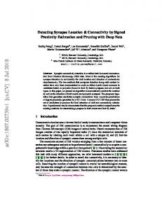
where the first two terms of this equation are irreducible error, and E N2 [(r(X2k−1 ) − r(X2k ))2 ] is the error from within pair differences in r(Xi ). If pairs do not match on the vectors Xi , but all pairs match on the scalars r(Xi ) then E N2 [(r(X2k−1 ) − r(X2k ))2 ] = 0, and equation 5 would only involve irreducible error. This provides some intuition for this paper’s main results. Other than Assumption 1 the proof of optimality required that treatment effects be independent of (X, ). A requirement, like this one, restricting the relationship between the conditional expectations of potential outcomes is necessary for matching based on the prognostic score to be optimal. Consider the following counter example where we do away with this type of requirement and allow E(Yi (1)|Xi = x) and E(Yi (0)|Xi = x) to be unrestricted. Let potential outcomes be deterministic functions of a univariate X, and let X take on the following values in a sample of four. The data could come from four draws from the functions in Figure 1. The assumptions in Propositions 2 and 3 imply that the average treatment effect conditional on covariates is constant for all values of the potential outcomes. In this counter example, that would require the graphs in Figure 1 to differ by at most a vertical shift. In this


15

E(Yi (1)|xi ) E(Y(0)i |xi ) xi i 1

1

1 1

4

2

2 2

9

3

3 3

2

4

4 4

Figure 1 Exampl e: Esti mates of E(Y (0)| X) and E(Y (1)| X) 15

E(Y (1)| X)

10

5

0

E(Y (0)| X)

−5

−10 0

0.5

1

1.5

2

2.5

3

3.5

4

4.5

xi

deviation from that assumption the optimal pairing depends on more than the order given by either conditional expectation function. Pairing on the prognostic score would pair units {1, 2} and {3, 4}, and Var(D|X) would be 52/16. Pairs matched on the predicted outcome for treatment would give {1, 4} and {2, 3}

16


with Var(D|X) of 37/16. The optimal pairs in this case are {1, 3} and {2, 4}, they give Var(D|X) of 36/16. 2.1. General solution to the matching problem. Without making any assumptions we have the following formula for the variance:

i var(D) N h 2 2 2 2 (θ = E(θ ) − θ + 2E(r(X ) ) + 2E Y (0)) + 2E( ) i i i 2 i i 2 2 N N

− (6)

2 X

[2E(r(X2k−1 )r(X2k )) + E(θ2k−1 Y2k (0)) + E(θ2k Y2k−1 (0))]

k=1

+

X1 h,k

4

[E(θ2k−1 θ2h−1 ) + E(θ2k−1 θ2h ) + E(θ2k θ2h−1 ) + E(θ2k θ2h )]

N N − − 1 θ2 2 2 This is derived in a web appendix. The second and third rows depend on the way pairs are matched. Let E(Yi (1)|Xi ) ≡ r˜(Xi ), and i ≡ Yi (1) − r˜(Xi ). Therefore θi = r˜(Xi ) + ˜ − r(Xi ) − i . We have that E(θi Yi (0)) = E(˜r(Xi )r(Xi )) − E(r(Xi )2 ) − E(i2 ), E(θi Y j (0)) = E(˜r(Xi )r(X j ))−E(r(Xi )r(X j )), and E(θi θ j ) = E(˜r(Xi )˜r(X j ))−E(r(Xi )˜r(X j ))− E(˜r(Xi )r(X j )) + E(r(Xi )r(X j )). Each of which are functions of X. Since the set of possible matches is finite then for every possible realization of X optimization of equation 6 can be done by exhaustive search over this set. 3. Matching in Practice In practice the conditional expectation function–also referred to as the ‘prognosis score’ (Hansen, 2008)–is not known and will have to be estimated with data. This data can come from any sample from the same population, for example a previous experiment, a


17

rich baseline survey, an existing observational study, or administrative data. This initial prediction can be based on many baseline covariates. Since we will be using covariates to predict the outcome of interest, the goal is to use them to make predictions with the best out of sample performance. To this end there are many model selection procedures available, such as, AIC, BIC, Lasso, or ridge regression. This paper provides some guidance on how to estimate the best predictors in the examples and compares their performance.

Figure 2 shows each of the steps present in the matching procedure. The process starts with collection of baseline covariates for the units in the experiment, in addition to collection of auxiliary (training) covariates and outcome data from the same population. Next the training data is used to estimate a prediction function. This function, coupled with the baseline covariates from the experiment group form the procedure’s predicted outcomes. Matched pairs are based on these predictions. The pair assignments are then operationalized as a set of pair indicators. Next, randomization produces a treatment variable. After the experiment is conducted, an outcome variable is measured. The analysis of this experiment, however, will use just the pair indicators, outcome, and treatment variable.

To build intuition for the procedure and to draw important distinctions, it is useful to compare the present method with well known propensity score methods. In practice, the two steps for optimal matched pairs randomization are analogous to matching procedures in observational studies based on the propensity score (Rubin, 1983). In the first step, rather than estimating a propensity score (which is the conditional probability of treatment), we estimate a ‘prognostic score’ (Hansen, 2008), which is a conditional expectation of the potential outcome absent the treatment. Both scores aggregate the information present in pre-intervention variables. But while the propensity score describes how observables influence selection into treatment, the prognostic score describes how observables influence the outcome.

18


Figure 2. How auxiliary data is used in Matched Pair Randomization Training

(X, Y)train

Data

Estimate Prediction Function

rˆ Randomize Baseline Covariates

Xexpr

Match Pairs on rˆ(Xexpr )

Mexpr

and Conduct

(Y, T, M)expr

Analysis Sample

Experiment Notes: This figure shows each step in the matching procedure. The process starts with the collection of baseline covariates, Xexpr , for the units in the experiment and auxiliary (training) data from the same population that contains baseline covariates and outcome, (X, Y)train . Next the training data is used to estimate a prediction function, rˆ. This allows the experiment baseline covariates to form a predicted outcome. Matched pairs are based on these predictions, rˆ(Xexpr ). The pair assignments are given by a set of pair indicators, Mexpr . Randomization produces a treatment variable T , and an outcome variable, Y, which is measured after the experiment is conducted. The analysis of the experiment will use (Y, T, M)expr .

Since treatment in this model is binary, the propensity score must usually be estimated with probit or logit models as these both account for the binary dependent variable. On the other hand, the prognostic score is not restricted in the same manner unless the outcome is also binary. In propensity score methods the second step would typically involve controlling for the propensity score non-parametrically. This can more generally include matching or blocking, as well as fitting flexible univariate functions. However in matched pairs


19

randomization, the second step is usually fixed6. That is, inference in the second second step is performed in one standard way. We describe this in the next section.

4. Inference in Matched Pair Randomization After randomization, both frequentist inference and randomization inference depend only on the actual strata chosen and not on estimated predicted values. Covariates are used to form predictions which are then used to choose pairs. Ex-post analysis is done conditionally on the chosen pairs; thus it is unaffected by the process used to pick pairs. However, so long as good predictors of the outcome are used, significant gains in efficiency will most likely be realized. A standard way to obtain the difference in means estimator is from the following linear regression model (Duflo et al., 2006), E(Yi j |T i j , M j ) = α + βT i j + δ j M j

(7)

where i indexes individuals, j indexes pairs, T i j is a treatment indicator, and M j is a pair indicator. Frequentist inference can be done using either the standard or robust estimates of the least squares variance. In the case of matched pairs, there is also another procedure available, i.e. the paired difference test (Rubin, 1973). The simplest way to think of the paired t-test is to construct within pair differences, D j ≡ Y1 j − Y2 j (indexed so that the first unit is treated). This gives one difference for each pair. The rest of the procedure amounts to estimating P the mean with the sample average of the differences, D = 1n j D j , where n is the number 6

Dierh et al (1995), Snedecor and Cochran (1979), and Lynn and McCulloch (1992) discuss ‘breaking the

matches’ ex-post in matched pair randomization and find that tests that ignore the procedure are conservative. ‘Breaking the matches’ is a hybrid design where one matches, but then analyses the data as if matching had not occurred.

20


of pairs. Standard errors for the test come from the appropriately normalized sample q 1 P 2 variances of the differences, SE= 1n n−1 j (D j − D) . A t-statistic, D/SE, is formed and compared to a critical value from the t-distribution with n − 1 degrees of freedom. The test can be justified either asymptotically given a central limit theorem holds or in finite samples with the assumption of normal errors. Thus given a matched pair randomization one can view the data as a set of N outcome measurements from the experimental units, where N/2 have been treated. One can then proceed with analysis by regressing the outcome on a treatment indicator alongside a set of N/2 pair indicators. Alternatively one can view the data as a set of n = N/2 within pair differences wherein the statistician is estimating the simple mean of the n within pair differences7. Randomization inference can also be conducted ex-post. The method, in general, considers a test statistic and a sharp null hypothesis. The test statistic is evaluated at all possible counter-factual assignments that could have been realized by the experiment. A sharp null hypothesis then specifies exactly what the treatment effect is for every experimental unit and allows counter-factual potential outcomes to be computed for every unit. It is commonly the case that the sharp null hypothesizes exactly zero effect of treatment for every unit. Under this null both potential outcomes are identical for each unit, so that outcomes would be the same under any treatment assignment. In a matched pairs experiment with N/2, pairs there would be 2N/2 possible assignments and the distribution of a test statistic can be computed over this distribution. Inference would then be conducted by comparing the value of the statistic to the proportion of more extreme values in the underlying distribution.

7

Two interesting but non critical observations are described in appendix A.


21

4.1. Treatment Compliance. Often in experiments not all treatment assignments are followed. For example experimenters may randomize admission into a work-training program, but not all admitted applicants may enroll. Furthermore, some applicants who were randomized out of the program may be admitted after reapplying. In these cases one can use the original treatment assignments to estimate the effect of Intent To Treat (ITT) by redefining T i in this model’s set-up to denote treatment assignment instead of actual treatment.

5. Model Selection and Prediction Methods In this section we present and discuss four model selection methods: AIC, the Akaike Information Criterion; BIC, Bayes’ Information Criterion; Lasso, the least absolute shrinkage and selection operator; and Ridge regression. This paper uses each of these four methods to select models in simulations.

5.1. AIC and BIC. The Akaike (1974) Information Criterion comes from a correction for over-fitting in a maximum likelihood model. In the likelihood model, this means that the Kullback-Leiber distance between the selected model and the true model is smaller than would be expected. The expected bias is then computed and the estimate is subtracted out. AIC is a transformation of the bias corrected distance between the true model and the given model. On the other hand, the Bayes’ Information Criterion (BIC) comes from a Laplace approximation of the probability of observing a given set of data conditional on a particular model. Both AIC and BIC have a long history of application in time series where one of the main questions is regarding how to select the order of AR and ARMA models (c.f. Shibata, 1976 and Brockwell and Davis, 2002). Researchers with access to long panel data sets, such as semester grades from kindergarten to tenth grade, may

22


find AR models useful for predicting class 11 grades. The methods noted above are more generally useful in classifying how well different models fit a dataset. We use the AIC in the case of independent identically distributed data. This derivation follows Claskens and Hjort (2008). Let Y1 , ..., Yn be i.i.d. from an unknown density g. Consider a parametric model with density fθ (y) = f (y, θ) where θ = (θ1 , ..., θ p )0 belongs to some subset of R p . MLE minimizes the Kullback-Leibler distance (KL) between the fitted and true model, KL =

Z

Z g(y) log g(y)dy −

ˆ g(y) log f (y, θ)dy.

The first term is constant across models fθ so consider Z ˆ Rn = g(y) log f (y, θ)dy. ˆ Now consider it’s expected This is a random variable, dependent on the data via θ. value Qn = Eg [Rn ] = Eg

"Z

# ˆ g(y) log f (y, θ)dy .

and estimate Qn from data via n

1X ˆ = 1 ln,max . log f (Yi , θ) Qˆ n = n i=1 n We can show that Qˆ n is higher than Qn on average, and the bias is

E(Qˆ n − Qn ) ≈ p∗ /n,

where p∗ = trace(J −1 K)

where " J = −Eg

# ∂2 log f (Y, θ0 ) , ∂θ∂θ0

" K = Varg

# ∂ log f (Y, θ0 ) . ∂θ

If g = fθ0 then J = K. A bias-corrected estimator of Qn is Qˆ n − p∗ /n = (1/n)(ln,max − p∗ ).


23

When the model actually holds, i.e. g(y) = f (y, θ0 ), then K = J is the Fisher information matrix of the model, and p∗ = tr(J −1 K) = p = dim(θ). If we take p∗ = p, the number of parameters in the model, this gives the AIC criterion AIC = −2ln,max + 2p In the normal linear model Yi |xi ∼ N(xi β, σ2 I) we have that −2ln,max = nlog( S Sn R ), where P S S R = ni=1 (ˆyi − y)2 so AIC = n log( S Sn R ) + 2p. The BIC comes from comparing the posterior probability that a model is the true model. We have that M1 , M2 , ... are potential models. The probability that data come from model M j given the observation of data, Y, is P(M j ) P(M j |Y) = f (Y)

Z Θ

f (Y|M j |θ)π(θ|M j )dθ

where P(M j ) is the prior probability that data come from M j , and f (Y) is the unconditional likelihood of observing data Y. For selecting among models using the same data, f (Y) is fixed. We also give each model equal prior by fixing P(M j ). Now we can rewrite R f (Y|M j |θ)π(θ|M j )dθ as Θ Z 1 exp(n ln, j (θ))π(θ)dθ n Θ and apply a Laplace transformation to give the approximation ! p/2 h i 2π 1 exp(n ln, j (θ)) π(θ)|J(θ)|−1/2 n n = (2π) p/2 n−p/2 f (Y|M j )π(θ)|J(θ)|−1/2

24


where p is the dimension of the parameters in model j. The BIC that we use comes from the first two dominant terms after taking the log of this expression. Taking the log gives

p 1 p log(2π) − log(n) + ln, j (θ) + log(π(θ)) − log|J(θ)| 2 2 2 and the two dominant terms are p − log(n) + ln, j (θ) 2 since they get arbitrarily large with n. The BIC for model j is this expression multiplied by −2. BIC = p log(n) − 2ln, j (θ). For the normal linear model we have that BIC = n log

S S R n

+ p log(n).

Models are compared with BIC or AIC by taking the set of models under consideration, and then computing AIC and BIC values for each one. Since the penalty term p log(n) is higher for BIC than for AIC (which has a penalty of p2), BIC will have a tendency to select lower dimensional models. As the number of models grows large, evaluating each model individually becomes burdensome. In the next section we turn to model selection methods that choose models without the need to compute a value for each. 5.2. Ridge and Lasso. Ridge and Lasso are methods that select from many possible models simultaneously. Here we describe Lasso and Ridge and follow Hastie, Tibshirani, and Friedman (2009). Although more amenable to large parameter spaces (models can be estimated with more covariates than observations), Ridge and Lasso are defined for linear models. Instead of introducing a penalty term after model parameters have been estimated,


25

these shrinkage methods include a penalty within a modified least squares optimization problem. Solving the optimization problem produces the best model. For comparison recall the OLS estimator βˆ = arg min(y − xβ)0 (y − xβ) β

where y is an N × 1 vector of outcomes, x is a N × k matrix of covariates that includes a constant in the first column, and β is a k × 1 parameter vector. Let us decompose the covariates into the constant and the remaining columns x = [1, x˜], and let us do the same for the parameters β = (β0 , β˜ 0 )0 . Now we can write down the ridge estimator as h i arg min (y − xβ)0 (y − xβ) + λβ˜ 0 β˜ . β

Instead of minimizing the sum of squared residuals as in OLS, the Ridge estimator is minimizing the sum of squared residuals plus a linear penalty in the sum of the squares of the coefficients. One drawback of this method is that changes in the scale of the inputs have non-trivial effects on the estimand. This paper follows standard practices and normalizes covariates to have mean zero and variance one before we estimate both Ridge and Lasso models. Ridge can also be reconciled in the following Bayesian model. Let yi ∼ N(xβ, σ2 ) i.i.d. for all i and let β j ∼ N(0, τ2 ) i.i.d. for all j. Then the posterior density of β with σ and τ known is i! 1 h 0 0˜ ˜ f (β|y, x) ∝ exp − 2 (y − xβ) (y − xβ) + λβ β 2σ where λ = σ2 /τ2 8. 8

This Bayesian interpretation of the Ridge model suggests a two step procedure as an alternative to

the standard practice of normalizing the variance of covariates to one. In the first step, if k < N one can orthonormalize the covariates and estimate the full model to obtain measures of the precision of the coefficients and an initial measure of σ. In the second step Ridge is estimated with λ set to σ2 .

26


Lasso follows a similar optimization to Ridge but changes the penalty so that it is linear in the sum of absolute deviations of the coefficients instead of linear in the sum of the squares like Ridge. More formally the estimator is described by   k X   0 arg min (y − xβ) (y − xβ) + λ |β j | . β j=1

The effect of changing the penalty on estimated coefficients is substantial. Lasso can produce models with coefficients set to zero. In this way, it can be interpreted as doing subset selection over the set of covariates. Ridge and Lasso estimates will depend on the magnitude of the penalty coefficient, λ. Our choice of this parameter starts by estimating models for various values of λ. For each model we estimate the mean squared error using ten-fold cross validation, then we chose the value λ with the lowest estimated mean squared error.

6. Data and Simulations 6.1. Dataset descriptions. Using data from Bruhn and McKenzie (2011), I conduct simulations in six cases. In some cases, the data come from actual field experiments. In others, the data is observational and the outcome and baseline variables are chosen to represent a hypothetical field experiment. Data come from four sources: Mexico’s national labor survey, a Sri Lankan micro-enterprise survey, a Pakistan education survey, and Indonesia’s Family Life survey. Table 1 gives summary statistics for variables in the six samples. The Mexican survey has data on monthly income9 and weekly work hours for households surveyed by the Mexican Encuesta Nacional de Empleo (ENE). This was Mexico’s national labor survey from 1988 to 2005. The ENE sample we use is for household heads between 20 and 65 who were first interviewed in the second quarter of 2002 and who were 9

Income is measured in pesos (MX$1=US$0.1)


27

reinterviewed in the next four quarters. We keep only those at the initial interview and imagine a treatment aimed at increasing their income. Sri Lankan data is on small enterprises and measures monthly profits and sales, weekly work hours, capital assets, demographic information on the business owner, and whether the business was affected by the 2004 Indian ocean earthquake and accompanying tsunami. Data collection was done in 2005 by De Mel, McKenzie, and Woodruff (2008), who also randomly assigned grants of 10,000 or 20,000 rupees (LKR) to Sri Lankan microenterprises. They surveyed firms with less than 100,000 LKR (US$1,000) in capital other than land and buildings. We imagine an experiment aimed at increasing firm profits. The sample of micro-enterprise firms is roughly evenly split between retail sales and manufacturing. Retail firms tend to be small grocery stores. Manufacturing firms range from clothing manufacturing to bicycle repair. The household asset index is the first principal component of a set of indicators or ownership of durable assets10. The Capital variable measures the value of assets in the firm excluding land and buildings. We run simulations in two cases with data on test scores and child height from Pakistan (Andrabi et al., 2008). Andrabi et al. study teacher value added estimates with three years of data from the Learning and Educational Achievement in Punjab Schools (LEAPS) project, an ongoing survey of learning in Pakistan. The sample comes from 112 villages in 3 Punjabi districts. Villages were chosen from the set of villages with at least one private school. Thus the sample has higher income and more education than the average rural village in the districts. The initial panel consisted of 13,735 third graders who were tested in Urdu, math, and English. These children were subsequently tested in fourth and fifth grade. We use a subsample of 6,379 children who were additionally surveyed on 10

The asset index uses seventeen indicators: cell phone; land-line phone; household furniture; clocks and

watches; kerosene, gas or electric cooker; iron and heaters; refrigerator or freezer; fans; sewing machines; radios; television sets; bicycles; motorcycles; cars and vans; cameras; pressure lamps; and gold jewelry.

28


anthropometrics (height, weight) and detailed family characteristics. Variables include a family wealth index, an indicator for having a high education mother, and district private school dummies. Math test scores are given as “knowledge scores” which range from zero to 1000 on the LEAPS exam. The variable wealth index is from a principal component analysis of twenty household assets. The last dataset comes from the Indonesian Family Life Survey (IFLS), an on-going longitudinal survey in Indonesia. The first wave was conducted jointly in 1993 by RAND and Lembaga Demografi, University of Indonesia. We use data from 1997 and 2000, the second and third waves respectively. In one sample we use children in 6th grade during the first survey and simulate a survey that keeps them in school. Our outcome is Child Schooling, an indicator for whether the child was in school in 2000. In the second sample we use household per capita expenditure data as an outcome and simulate a treatment that increases this outcome variable for households. The variable Household expenditure represents the log of household expenditures per capita. 6.2. Data generating process. In order to allow an arbitrary number of draws to be taken, and so that the true data generating process is known and can be used as a benchmark for each dataset, I first regress the outcome on a set of covariates chosen by Bruhn and McKenzie (2011)11. Next, I take the estimated coefficients and the mean squared error from this regression in each dataset and treat these estimates as the true parameters, (β, σ2 ) in a normal linear model y|x ∼ N(xβ, σ2 I). Tables 2 and 3 describe the regressions used for the data generating process and present the coefficients and MSE for each dataset. To generate observations I draw covariate vectors xi from those that are in the BM samples. That is, I take the joint distribution of xi , F x , to be the sample distribution in the BM data. 11

Bruhn and McKenzie call these “balancing variables” and each of the six datasets has seven of these

covariates. Each dataset from Bruhn and McKenzie (2011) has three hundred observations.


29

A simulated experiment draws two independent samples from this distribution, a training sample and an experiment sample. With the experiment sample it estimates prediction functions using the four methods from section 5, AIC, BIC, Ridge, and Lasso. Ridge uses ridge regression (Tibshirani, 1996) where the penalty term is chosen to minimize the mean squared error under ten-fold cross validation. LAS S O uses the least absolute shrinkage and selection operator (Tibshirani, 1996) where the penalty term is chosen to minimize the mean squared error under ten-fold cross validation. AIC uses the model among the 27 sub-models that has the lowest value of the Akaike information criterion (Akaike, 1974). BIC uses the model among the 27 sub-models that has the lowest value of the Bayes information criterion (Schwarz, 1978). In each of the four methods the full model is linear in a constant and the seven “balancing variables” and corresponds to the data generating process. After this is done the training data is discarded and only the estimated prediction functions are kept. These are used to form predictions of the outcome in the experiment sample. We investigate how matching pairs according to the predicted outcome performs against complete randomization, and against matching pairs according to the baseline outcome12. We are interested in the lagged outcome because this covariate is highlighted by Bruhn and McKenzie and performs well in their simulations. For matching according to the predicted outcome we compare the four methods of forming predictions from section 5. Our benchmark estimates draw a training sample of 2000 observations of the outcome and covariates and form predictions for an independent placebo experiment sample of 100. For each method we report the mean squared error of the difference in means; we form .95 confidence intervals and report the proportion of estimates that fall outside the confidence

12

For the schooling outcome in the IFLS data set, since all children are in school at baseline we match on

mother’s level of education.

30


interval; lastly we estimate rejection probabilities (power) for plausible treatment effects in each experiment. A second set of simulations investigates how performance changes when we decrease the size of the training sample. Finally two additional sets of simulations investigate the same measures of performance when we first decrease then increase the size of the experimental sample. This is motivated by findings from BM who observe smaller gains from matching with samples sizes of 300 and above.

6.3. Benchmark performance. Table 4 shows the relative mean squared error from each method in our benchmark case. In this first set of simulations the size of the training sample is 2000, the size of the experiment sample is 100, and the number of simulations per dataset per method is 10,000. We call a training sample of 2000 and an experiment of 100 the benchmark case. The values in table 4 are scaled so that, for each data set, the mean squared error under complete randomization is one. For example, row 1 column 3 implies that the mean squared error using matched pairs and matching using the predicted value from Ridge regression produces mean squared error that is .748 times the size of the mean square error under complete randomization.

6.4. Choice of matching variable. Generally in table 4, matching on the predicted values does better than matching the lagged values of the outcomes. In these datasets, matching on the lagged values of the outcome produces mean squared errors that are the about the same size or 2 percent smaller than complete randomization. Note that the biggest improvement comes from dataset 3 and that the least improvement comes from dataset 2. This is in line with the predictive power i.e. R2 , from the data generating process. The gain in mean squared error relative to complete randomization is 1 − R2 and dataset 3 has the highest R2 while dataset 2 has the lowest R2 .


31

6.5. Are standard errors the correct size? Table 5 considers whether tests using the various randomization methods have correct size. This is a first order concern before efficiency gains are considered. That is whether .95 confidence intervals formed following the linear regression model in equation (1) reject the null of no effect when there is in fact no effect of treatment. Table 5 shows that across all methods, size is well controlled. Rejection rates over 10000 simulations stay very close to .05 with the highest deviation to .055 and the lowest to .046. Table 6 compares the methods under plausible treatment effects. The effects for each method are described in the first column of the table. BM chose these treatment effects to be relatively small in magnitude so that differences can be seen in power across randomization methods. 6.6. Performance with smaller training set. Tables 7 to 9 in Appendix C present simulation results that move from the benchmark case and reduce the size of the training set from 2000 to 100. As one would expect we see in Table 8 that size continues to be controlled well across datasets and randomization methods. Table 7 shows that the reductions in mean squared error are about the same as in the benchmark case. For Math test scores (Pakistan) matching pairs reduces MSE by forty to forty-three percent with a training sample of 100. With a training sample of 2000 the Pakistani Math test score simulation produced reductions in MSE of about the same size. Table 9 shows that increases in power are about the same as in the benchmark case or slightly smaller. For the Mexican Labor income simulation with a smaller training sample, power under matching based on predicted outcomes gives results between .178 and .183. However in the benchmark case with a training sample of 2000, power is between .186 and .190. 6.7. Performance in small experiments. Tables 10 to 12 present simulations that move from the benchmark case and instead reduce the size of the units in the experiment from

32


100 to 30. Table 10 shows that this does cause a noticeable attenuation of the reductions in MSE relative to the benchmark case. In the benchmark case with the strongest reduction in MSE, i.e. the math test score example with Pakistani data, MSE drops by 40 percent with 30 experimental units. The reduction was .44 percent with Lasso in the benchmark case. Table 14 shows that tests still correctly reject 5 percent of samples when no treatment effect is present. By far, the biggest differences from the benchmark case come with respect to losses in the level of power from the reduction of sample size, relative to the benchmark case. The degrees of freedom reduction from the matched pairs method becomes an issue in Table 12. While power remains as high as complete randomization for methods that match on the predicted outcome, for matching on the lagged value of the outcome 4 of 6 datasets show lower power under matching on the lagged value of the outcome. 6.8. Performance in large experiments. The next case we consider takes the benchmark case and increases the size of the experiment to 300. Recall that the previous case reduced this sample to 30. Therefore, between the previous case of 30, the benchmark case of 100, and this case of 300 once can observe the performance of randomization methods over a tenfold increase in sample size. Tables 13 to 15 present results on MSE, size control and power. Comparing the relative MSE results in table 13 to 4 and 10 we see that the relative reduction in MSE is remarkably stable across sample sizes. Taking for example the intervention on Pakistani math test scores, there remains a forty percent reduction in mean squared error from complete randomization to either one of the four methods that match on the predicted values of the outcome. This performance is remarkably similar to tables 4 and 10. In similar simulations on math test scores, Bruhn and McKenzie find that the 95th percentile of the difference in means go from 0.23 to 0.17 as the randomization methods goes from complete randomization to matched pairs. They compare this to sample sizes of 30 where the reduction in this statistic is from 0.72 to 0.36. There are at least three reasons


33

for the discrepancy, (1) the statistic they report is different from the MSE reported here, (2) they match pairs using the Mahalanobis distance as a metric and the Greedy algorithm for selection, (3) each of their simulations uses the same sample of 30 and the same sample of 300 observations in terms of both outcomes and covariates. Each of these three could play a role. It is not obvious that relative percentiles of the distribution should scale proportionately with sample size. Furthermore the 95th percentile of the sampling distribution of the estimator may be a more important statistic than its mean square error. It is less likely that the Mahalanobis metric would play a significant role in the discrepancy, but how this balances covariates should be studied further. More worrisome is that a single sample of 30 was repeatedly used in the BM simulations. If the balancing variables had more predictive power for that sample than for the remaining sample of 270 that then this could lead to the dramatic differences that BM observes. 7. Literature The optimization problem of exhaustively paring subjects from a common pool is called optimal non-bipartite matching (Papadimitriou and Steiglitz, 1998). It has previously been taken up by Greevy et al (2004). The general staring point, if the total number of units is N, is an N × N matrix that holds a weakly positive real valued measure of distance between each subject. Greevy et al (2004) use the Mahalanobis distance (MD) metric suggested by Rubin (1979) in this matrix. Distances are then summed for each candidate set of pairs, and the set with the lowest sum is chosen. Under MD if x p,1 and x p,2 are the vectors of covariates for the two units of the pth pair, p = 1, ..., N2 , and Cˆ is an estimate of Cov(X), then the sum of within pair Mahalanobis distances is (8)

N q 2 X (x p,1 − x p,2 )Cˆ −1 (x p,1 − x p,2 )0 .

p=1

34


One can set x p,i to the covariates themselves, or to their ranks to minimize the influence of outliers. It is commonly suggested that covariates be normalized by setting means to zero and variances to one. One, benefit of weighting by the inverse covariance matrix is that covariates that are highly correlated will be given less collective weight and covariates that are orthogonal to the rest are given greater weight. This captures the problem of over counting covariates that are very similar. Greevy et al (2012) extends this method to incorporate missing data dummies, and pre and post multiplying C −1 by a matrix of user specified weights. The method in this paper uses the conditional expectation function to weigh covariates. Thus missing covariate values do not pose a problem since conditional expectation functions are comparable and can be constructed for any set of covariates. If there were fewer observed covariates for a particular observation then a conditional expectation function that uses just the non-missing variables as its argument can be estimated. For example, in the extreme case, if one particular experimental unit has no covariate information, then the best prediction of the outcome for this unit is the mean of the outcome.

While the Mahalanobis distance solves a well-posed optimization problem, it leaves much to be desired. Experimenters must choose which variables to include and in what functional form to include them. For example, the number of years of labor market experience can be included, as can the square of experience. Greevy et al (2004) suggest that covariates that matter for the outcome be chosen, but they go no further. If many irrelevant covariates are included in addition to strong predictors then this method will produce less of a gain than if the irrelevant variables were excluded. Matching on the predicted outcome (as is done in this paper) is not immune from the selection of an overly complex model. However, prediction is a richly studied concept in model selection, forecasting, machine learning and computer science, and there are many suggested solutions to resolve


35

the issue of over-fitting. Thus if many irrelevant covariates are included among the set of predictors, those covariates will be given very little weight or excluded completely. Two very notable contributions to the experimental design literature from within the field of economics are Hahn et al. (2011) and Kasy (2012). Hahn et al’s method requires at least two experiments. The first experiment is conducted with complete randomization, and the data from that experiment are used to compute estimates of the conditional variance, Var(Yi (t)|Xi = x), where t ∈ {0, 1} is realized treatment, and Yi (·) is a potential outcome function. In principle, conditional variances for untreated potential outcomes could also be estimated in observational data. From these estimates the optimal treatment probabilities (propensity scores) p(x) ≡ Pr(T i = 1|Xi = x) are computed and used in subsequent experiments. In the end inference is done by pooling the data from all the experiments. The optimization minimizes the asymptotic variance of the average treatment effect. Hahn et al. consider the two-step estimator proposed by Hirano, Imbens, and Ridder (2003) and others ! N X T i Yi (1 − T i )Yi ˆβ = 1 − . N i=1 p(X ˆ i ) 1 − p(X ˆ i)

(9)

This estimator achieves the asymptotic variance bound given by Hahn (1998). In a matched pairs design pˆ is set to

1 2

for all values of Xi . Hahn et al (2011) consider assignment prob-

abilities as a function of each unit’s own covariate values, Xi . This rules out a method like stratification where the treatment assignment vector is a function of the joint set of covariates X = (X1 , ..., XN )0 . Their method is an extension of the Neyman allocation formula (Neyman, 1934), where variance is now conditioned on covariates as well as treatment status. One could possibly reconcile the approach with stratification by using estimates of the conditional variance. Using those estimates, one can compute optimal treatment probabilities as a function of the conditional expectation of the outcome. Then one can stratify

36


based on the conditional expectation where the relative number treated within each stratum is set to match the optimal treatment probability for the average covariate value of the stratum. Kasy (2012) formalizes the most balanced distribution of relevant characteristics across treatment groups and explicitly describes Bayesian and frequentist inference. The most balanced distribution of covariates is unique with probability 1 if the set of covariates includes at least one continuous covariate. Since randomization in general gives weight to assignments that are not the most balanced, efficiency gains can be had by not randomizing. The formal structure is Bayesian and implies an optimal assignment and best linear estimator. Frequentist inference can be conducted treating conditional potential outcomes as random given covariates and treatment. Frequentist inference, however, requires estimating the conditional variance. Kasy suggests first estimating the residuals ˆi = Yi − fˆi , where fˆ is a non-parametric Bayes estimator of the conditional expectation of the outcome. Then these residuals can be used to estimate the conditional variance. Within the stratification literature there are frequent recommendations on which variables to use. But guidance never goes beyond advocating for variables that are strongly related to the outcome. In particular there is an absence of recommendations on how to trade-off the balance between multiple variables that are either continuous or discrete with a large support. Here are some quotes from recommendations in the literature. • “Statistical efficiency is greatest when the variables chosen are strongly related to the outcome of interest (Imai et al., 2008).” • “Matching is most effective if the matching variable is highly correlated with the endpoint. In most cases, the closest correlation is likely to be with the baseline value of the same endpoint, and so this is a natural candidate for matching (Moulton and Hayes, 2009).”


37

• “The strength of the correlation within matched pairs or strata may be increased by matching on more than one variable, each of which is correlated with the endpoint (Moulton and Hayes, 2009).” • “This paired or blocked design produced a sizeable increase in information in comparison with the completely randomized design by reducing the noise (experimental error) affecting the estimation of the difference in the treatment means (Mendenhall, 1968).” • “Blocking on variables related to the outcome is of course more effective in increasing statistical efficiency than blocking on irrelevant variables, and so it pays to choose the variables to block carefully (Imai, King and Stuart, 2008).” • “Matching should lead to greater comparability of the intervention and control groups, and precision and power should be increased to the extent that the matching factors are correlated with the outcome” (Hayes and Bennett, 2009). This paper goes further than these suggestions by offering an explicit method for the choice of matching variables. Matched pair randomization has been studied extensively by statisticians. Mosteller (1947) and Mc Nemar (1949) studied inference with matched pairs where the response was binary. Each proposes a χ21 test conditional on the number of pairs whose responses do not match and testing the null that the probability of observing (0,1) and (1,0) is the same based on the normal approximation to the binomial distribution. Cox (1958) showed that in some cases the McNemar test is uniformly most powerful unbiased. Cox used a logistic model. Chase (1968) compares the efficiency loss from pairing on irrelevant X in models with a binary response.

38


Bruhn and McKenzie (2009), in simulations, find that pair-wise matching and stratification appear to dominate re-randomization. Re-randomization is the practice of constructing criteria for balance, then randomizing over the set of treatment assignments that meet the criteria. For example, Casey et al (2011) use as their criteria no statistically significant differences between treatment and control groups, in tests with size of five percent, on either of two covariates. Ex-post, Bruhn and McKenzie (2009) show that correct analysis can be done by including the covariates in regression analysis. McKinlay (1977) lays out several limitations of pair matching; in particular, the loss of sample from discarding control units in observational studies where the number of treatment units is smaller than the number of control units or when matches are hard to find. In our set-up neither of these things are possible because the number of control units is fixed at half the experiment sample and no units are discarded. Discarding units from a simple random sample would change the target parameter away from the ATE. Shipley, Smith and Dramaix (1989) calculate power in clustered and unclustered matched pair experiments. They focus on the t-test of the n/2 differences and give a formula for the power of a test of size α. If we let di be the ith within pair difference for i = 1, ..., m P where there are m total pairs, then d = mi=1 di /m, and the variance of d is estimated as P (di − d)2 /m(m − 1) . Power, the probability of rejecting the null when the true effect size is ∆ is given by 1 − β where β comes from cβ =

|∆|m1/2 SE(d)(m + 2)1/2

− cα/2

where c x denotes the value cutting off a portion x of the upper tail of the standard normal distribution. They give a similar formula for clustered randomizations where many individuals make up the unit of randomization. Lynn and McCulloch (1992) consider the case where experimenters have conducted a matched pairs randomization but will be ignoring the paired nature of the data in the ex-post analysis. In simulations they find that tests are


39

conservative when ignoring the matching. They also compare matching against ex-post regression to control for the influence of covariates. They set up a linear model but they consider the case where matching was exact for a set of variables. That is where a subset of covariates are identical within pairs.

7.1. Extensions to other randomization settings. Use of the prognostic score as a way of aggregating covariate information extends beyond the matched-pair setting. Here I explore two other randomization procedures where the prognostic score is useful and is a better aggregator of information than current standards. First I explore designs for sequential randomization as used in clinical trials and job training program evaluation. Next, I return to non-sequential experiments and discuss re-randomization methods. Designs for sequential treatment allocation over a span of time, as would occur in clinical trials, have been developed by Efron (1971) and others13. Efron (1971) suggests a biased coin design14. His aim is to balance the size of the treated and control groups within a discrete covariate category15. As an example consider four age categories. His method 13

White and Freedman (1978), Pocock and Simon (1975), Pocock (1979), Simon (1979), Birkett (1985),

Aickin (2001), Atkinson (2002), Scott et al. (2002), McEntegart (2003), and Rosenberger and Sverdlov (2008) are some in a very extensive literature that addresses various issues in sequential trials. In each case the problem is complicated by many covariates. 14 An upwardly biased probability rather than a completely deterministic assignment rule that places the new patient in the smaller control group of 16 to 25 year olds addresses a worry of having the experimenter bias treatment assignment. Efron (1971) notes that “If the experimenter knows for certain that the next assignment will be a treatment, or a control, he may consciously or unconsciously bias the experiment by such decisions as who is or is not a suitable experimental subject, in which category the subject belongs, etc.” 15

There are many extensions of this design. The most well known is Wei (1978) which has an adaptive

design that increases the bias with the magnitude of the difference is sizes between the treatment and control group.

40


tries to balance the number of treated and control subjects in each category. E.g. if there are more 16 to 25 year olds in the treatment group than in the control group and the next patient is 24 then that patient would be given a .6 probability16 of assignment to the control group and a .4 probability of assignment to the larger treatment group. Normally, in the biased coin design additional variables require an increase in the number of categories. Using the prognostic score here would be helpful since the number of categories would not increase with the number of covariates. Following Efron’s example with four age categories, the prognostic score could similarly be split into four categories, cutting at the quartiles of its distribution. Additional variables would change the amount of information represented in the prognostic score but not the four quartiles. A large number of categories in Efron’s sequential design motivated the Big Stick approach of Pocock and Simon (1975). They say, the “main difficulty” with methods like Efron’ is the rapid increase in strata as the number of covariates increases. Pocock and Simon’s method starts with choosing categories for covariates, like Efron (1971). The method then aggregates variation of covariates across treatment arms, and proceeds to aggregate information across covariates. This requires choices of simple aggregation functions at each stage that throw away covariate information. The prognostic score would be helpful here. If a prognostic score were used as the single covariate, then there would be no need to chose a function for ”the total amount of imbalance” in treatment numbers across covariates. In short section 3.2 of Pocock and Simon (1975) would not be needed, and, in the case of two treatment arms, the method would reduce to Efron’s biased coin design. Lock and Rubin (2012) suggests re-randomization and randomization inference in nonsequential trials. The method requires the researcher to designate a measure of covariate

16

In general this can be any probability greater than 1/2.


41

balance. They consider the Mahalanobis distance as a re-randomization criterion. A randomization is deemed acceptable whenever the Mahalanobis distance between the treatment and control groups falls below a certain threshold. The method in this paper suggests an alternative distance measure that is more directly related to the outcome of the experiment. We suggest using the predicted difference in average outcomes. The intuition for how the predicted outcome and the Lock and Rubin (2012) procedure are complimentary uses the same intuition as before. The predicted outcome function collapses the covariate space into one dimension, so once can use this single covariate in Lock and Rubin. The Mahalanobis distance with a single covariate is exactly the average difference in the covariate.

8. Conclusion This paper discusses how stratification can be done so that the variance of the difference in means is minimized. We show that in a matched pairs setting, the variance of the difference in means is minimized when pairs are chosen according to their predicted outcome. That is the prediction of the outcome as a function of baseline covariates. We show that the optimal predictor is the minimizer of the mean squared error, i.e. the conditional expectation function. Here we only consider strata that are pairs and where there is exactly one treated unit and one control unit in each pair. The main result is that pairs should be assigned by ranking units according to their predicted outcome. It remains to be seen whether this result holds for larger strata, for situations where there are different numbers of treated and control units, and more than two treatment arms. This method seems fruitful to examine in other settings too. Future research can extend the results here to the more general stratification problem.

42


Another avenue for further research is to examine alternative optimality criteria. Minimizing the mean squared error of the difference in mean outcomes naturally aligns with forming predictions of the outcome according to the conditional expectation function. Minimizing the mean absolute value of the error might lead to optimal matching based on predictions of the outcome using the conditional median function. Similar optimization problems involving quantiles of the distribution of the difference in means can also be examined. These may lead to a more direct way of increasing power of tests. The formula derived in Proposition 1 can be used in power calculations; at the point of randomization the experimenter, as we have seen, can estimate the function r and E( 2 ). Since baseline variables Xi are also known then one can calculate power treating r as known for various stratifications or other experimental designs.


43

Table 1. Dataset Descriptions Variable name

Mean

SD

Variable name

Labor income (Mexico, ENE)

Mean

SD

Height z-scores (Pakistan, LEAPS)

Labor income

4.33e+03 4.93e+03 Height z-score

-0.28

1.17

Baseline income

4.56e+03 5.4e+03

Baseline height

-0.162

1.21

Hours worked

48.1

14.1

Baseline weight

-0.581

0.991

Female dummy

0.13

0.337

Female dummy

0.443

0.498

Rural dummy

0.27

0.445

Wealth index

-0.0962 1.72

Number of rooms in home

3.83

1.5

High educ. mother dummy

0.223

0.417

Business owner dummy

0.35

0.478

District 1 dummy

0.303

0.46

1 to 5 employees dummy

0.507

0.501

District 2 dummy

0.31

0.463

Microenterprise profits (Sri Lanka)

Household expenditures (Indonesia, IFLS)

Microenterprise profits

5.77e+03 8.22e+03 Household expenditure

12.3

0.766

Baseline profits

3.9e+03

3.5e+03

Urban dummy

0.48

0.5

Hours worked

52.2

22

Household size

4.53

2.19

Female dummy

0.477

0.5

Male household head dummy 0.827

Baseline sales

1.18e+04 1.53e+04 Age of household head

47.7

14.9

Capital

2.63e+04 2.65e+04 Years educ. household head

5.29

4.3

Asset index

0.198

1.77

Baseline h.hold expenditure

12.3

0.74

Tsunami dummy

0.26

0.439

Number of children below 5

0.537

0.755

Math test scores (Pakistan, LEAPS)

0.379

Child schooling (Indonesia, IFLS)

Math test score

545

171

Child Schooling

0.737

0.441

Baseline math score

508

155

Age

12.4

1.16

Baseline english score

501

166

Female dummy

0.513

0.501

Age

9.65

1.06

Govt. school dummy

0.83

0.376

Female dummy

0.487

0.501

Mothers educ.

4.73

4.03

Wealth index

0.174

1.74

Urban dummy

0.48

0.5

High educ. mother dummy 0.243

0.43

Household size

5.5

1.62

Private school dummy

0.465


12.3

0.747

0.313

Notes: This table describes the datasets used in our simulations. Each dataset contains 300 observations. The first row of each panel describes the variable we treat as the outcome in out simulations. The next seven rows describe variables we use as covariates. The models are linear in these covariates.

44


Table 2. Dataset Descriptions Labor income (Mexico) Constant

2213.82

Microenterprise (Sri Lanka) Constant

(1165.17) Baseline income

0.433

Female dummy

Rural dummy

4.65

Baseline profits

Hours worked

(21.81)

-1.15e+03 Female dummy

-115

(740.63)

(959.90)

-1.17e+03 Baseline sales

0.036

(568.57)

(0.03) Capital

156

-353

Baseline math score

0.041

Asset index

84.3

Baseline english score

(691.98)

0.107 (0.07)

Age

-3.95 (7.19)

Female dummy

-32.1 (15.37)

Wealth index

-0.143 (4.77)

High educ. mother dummy -5.21

(280.87) Tsunami dummy 749

0.581 (0.06)

(0.02)

(742.99) 1 to 5 employees dummy

35.6

236.50 (77.29)

(0.15)

(178.48) Business owner dummy

0.441

(17.23)

Number of rooms in home 132

Constant

(1439.47)

(0.05) Hours worked

547.00

Math test (Pakistan)

(17.98) Private school dummy

(1039.68)

46.8 (19.59)

F stat

17.31

F stat

5.81

F stat

32.19

Ad. R2

0.280

Ad. R2

0.100

Ad. R2

0.420

Root MSE

4190.740

Root MSE

7789.430

Root MSE

129.700

Notes: This table describes the datasets used in our simulations. Each dataset contains 300 observations. Each column in this table describes a regression of that data set’s outcome on a constant term and seven covariates. Coefficients are reported with standard errors in parentheses. The coefficients from these regressions and the root mean squared error were used to define part of the data generating process for each simulation. The data generating process is completely described by noting that we use the joint empirical distribution of the covariates to draw observations.


45

Table 3. Dataset Descriptions (cont) Height z-score (Pakistan) Constant

-0.27

Household Exp. (Indonesia) Constant

(0.11) Baseline height

0.46

0.106

Urban dummy

0.25

Household size

-0.04

Male household head dummy

-0.15

Age of household head

-0.12

Years educ. household head

0.261


Ad. R

22.77 2

Root MSE

-0.214

0.001

0.048

0.356

Number of children below 5

-0.105

Govt. school dummy

16.42 2

0.138 (0.06)

Mothers educ.

0.025 (0.01)

Urban dummy

0.095 (0.05)

Household size

-0.017 (0.01)


(0.06) F stat

0.021 (0.05)

(0.06)

(0.14) F stat

Female dummy

(0.01)

(0.14) District 2 dummy

0.004

(0.02)

(0.01)

(0.14) District 1 dummy

-0.055

(0.11)

(0.03) High educ. mother dummy

Age

(0.02)

(0.11) Wealth index

-0.006

0.54 (0.52)

(0.07)

(0.08) Female dummy

Constant

(0.77)

(0.07) Baseline weight

7.88

Child Schooling (Indonesia)

0.056 (0.03)

F stat

8.34 2

0.340

Ad. R

0.270

Ad. R

0.950

Root MSE

0.660

Root MSE

0.150 0.410

Notes: This table describes the datasets used in our simulations. Each dataset contains 300 observations. Each column in this table describes a regression of that data set’s outcome on a constant term and six covariates. Coefficients are reported with standard errors in parentheses. The coefficients from these regressions and the root mean squared error were used to define part of the data generating process for each simulation. The data generating process is completely described by noting that we use the joint empirical distribution of the covariates to draw observations.

46


Table 4. Mean Squared Error for Multiple Randomization Methods Ntrainingsample = 2000, Nexperiment = 100

Randomization Method CR

MPY0

MPYˆ Ridge

MPYˆ LAS S O

MPYˆ AIC

MPYˆ BIC

MPYˆ orcl

Labor income (Mexico)

1.000

1.036

0.750

0.735

0.755

0.760

0.752


1.000

0.985

0.871

0.891

0.851

0.850

0.840

Math test score (Pakistan)

1.000

1.003

0.586

0.578

0.566

0.566

0.567

Height z-score (Pakistan)

1.000

1.013

0.670

0.642

0.682

0.675

0.647

Household expenditures (Indonesia)

1.000

0.998

0.711

0.732

0.747

0.776

0.720

Child schooling (Indonesia)

1.000

1.001

0.833

0.823

0.821

0.835

0.830

Notes: This table gives mean squared error estimates relative to complete randomization. CR is complete randomization, that is, under no stratification. MPY0 is matching on the lagged value of the outcome in each dataset. The next four columns MPYˆ x match pairs according to the predicted outcome, where the prediction is formed from a training dataset using method x. Ridge uses ridge regression (Tibshirani, 1996) where the penalty term is chosen to minimize the mean squared error under ten-fold cross validation. LAS S O uses the least absolute shrinkage and selection operator (Tibshirani,1996) where the penalty term is chosen to minimize the mean squared error under ten-fold cross validation. AIC uses the model among the 27 sub-models that has the lowest value of the Akaike information criterion (Akaike, 1974). BIC uses the model among the 27 sub-models that has the lowest value of the Bayes information criterion (Schwarz, 1978). In each of the four methods the full model is linear in a constant and the seven “balancing variables” and corresponds to the data generating process. The size of the the training sample used to estimate these predictors is Ntrainingsample = 2000 and the total number of unit in each simulated experiment is Nexperiment = 100.


47

Table 5. Size control for Multiple Randomization Methods Ntrainingsample = 2000, Nexperiment = 100


MPY0

MPYˆ Ridge

MPYˆ LAS S O

MPYˆ AIC

MPYˆ BIC

MPYˆ orcl


0.047

0.054

0.048

0.050

0.049

0.048

0.048


0.051

0.052

0.052

0.055

0.047

0.047

0.046


0.054

0.049

0.047

0.052

0.047

0.048

0.051


0.049

0.049

0.054

0.048

0.052

0.052

0.048


0.052

0.052

0.051

0.055

0.050

0.051

0.050


0.050

0.050

0.052

0.051

0.052

0.050

0.048

Notes: This table gives the rejection rates for .95 significance tests using multiple randomization methods. The randomization methods and sample sizes are described in Table 4.

Table 6. Power for Multiple Randomization Methods Ntrainingsample = 2000, Nexperiment = 100

Randomization Method TE

CR

MPY0

MPYˆ Ridge

MPYˆ LAS S O

MPYˆ AIC

MPYˆ BIC

MPYˆ orcl


0.17

0.149

0.151

0.180

0.185

0.177

0.184

0.187


0.12

0.096

0.093

0.099

0.100

0.093

0.095

0.092


0.22

0.196

0.200

0.295

0.311

0.302

0.304

0.308


0.25

0.250

0.243

0.345

0.330

0.338

0.334

0.350


0.51

0.716

0.709

0.847

0.840

0.817

0.817

0.841


0.24

0.225

0.218

0.248

0.240

0.235

0.241

0.251

Notes: This table gives the rejection rates for .95 significance tests, under the treatment effect given under column T E, using multiple randomization methods. The treatment effects are presented as standard deviations of the outcome variable. The randomizations methods and sample sizes are described in Table 4.

48


References [1] Aickin, Mikel. (2001). “Randomization, Balance, and the Validity and Efficiency of Design-Adaptive Allocation Methods.” Journal of statistical Planning and Inference, 94(1): 97Ð119. [2] Akaike, Hirotugu (1974) “A new look at the statistical model identification”, IEEE Transactions on Automatic Control 19(6): 716-723 [3] Altham, Patricia (1971) “The analysis of matched proportions" Biometrika 58, 3 pp561 [4] Altman, Douglas G. (1985) “Comparibility or Randomized Groups” Journal of the Royal Statistical Society. Series D (The Statistician) Vol 34 No 1pp. 125-136 [5] Andrabi, Tahir, Jishnu Das, Asin Khwaja, and Tristan Zajonc (2008) “Do Value-added Estimates Add Value? Accounting for Learning Dynamics” American Economic Journal: Applied Economics, 3(3): 29-54 [6] Angrist, J., J. Pischke (2010) “The Credibility Revolution in Empirical Economics: How Better Research Design is Taking the Con out of Econometrics” Journal of Economic Perspectives 24(2): 3-30 [7] Angrist, J., G. Imbens, and D. Rubin (1996) “Identification of causal effects using instrumental variables,” Journal of the American Statistical Association 91, 444-455. [8] Angrist, J., Sarah Cohodes, Susan Dynarski, Parag Pathak, and Christopher Walters (2013) “Stand and Deliver: Effects of Boston’s Charter High Schools on College Preparation, Entry, and Choice” NBER Working Paper 19275 [9] Atkinson, A. C. (2002) “The comparison of designs for sequential clinical trials with covariate information. Journal of the Royal Statistical Society, Series A 165 349-373 [10] Beshears, John, James Choi, David Laibson, Bridgitte Madrian, Katherine Milkman (2011) “The Effect of Providing Information on Retirement Savings Decisions” NBER Working Paper 17345 [11] Birkett, N. J. (1985) “Adaptive allocation in randomized controlled trials” Control Clin Trials 6 146155 [12] Bloom, Nicholas, James Liang, John Roberts and Zichung Jenny Ying (2013) “Does working from home work? Evidence from a Chinese experiment” NBER Working Paper 18871 [13] Box, G., S. Hunter and W. Hunter (2005), Statistics for Experimenters: Design, Innovation and Discovery, Wiley, New Jersey. [14] Brockwell, P.J. and R.A. Davis (2002) Introduction to Time Series and Forecasting (2nd edition). Springer-Verlag, New York


49

[15] Bruhn, M., and D. McKenzie (2008), In Pursuit of Balance: Randomization in Practice in Development Field Experiments, mimeo, World Bank. [16] Casey, K., and R. Glennerster, and E. Miguel (2012) “Reshaping Institutions: Evidence on Aid Impacts Using a Preanalysis Plan” Quarterly Journal of Economics 127 (4): 1755-1812 [17] Chaloner and Verdinelli (1995), ÓBayesian Experimental Design: A Review, Statistical Science 10(3), 273-304 [18] Chase G.R. (1968) “On the efficiency of matched pairs in Bernoulli trials" Biometrika, 55, 365-9 [19] Cochran W. G. (1950) “The Comparison of Percentages in Matched Pairs" Biometrika vol 37 no 3/4 dec pp 256-266 [20] Cox D. R. (1958) “Two further applications of a model for binary regression" Biometrika 45 562-5 [21] Cox, D., and N. Reid (2000), The Theory of the Design of Experiments, Chapman and Hall/CRC, Boca Raton, Florida. [22] De Mel, Suresh, David McKenzie, and Christopher Woodruff (2008) “Returns to capital: Results from a randomized experiment,” Quarterly Journal of Economics123(8) 1329-72 [23] Diehr, P., D. Martin, T. Koepsell, and A. Cheadle, (1995), Breaking the Matches in a Paired t-Test for Community Interventions when the Number of Pairs is Small, Statistics in Medicine Vol 14 1491-1504. [24] Donner, A. (1987), “Statistical Methodology for Paired Cluster Designs”, American Journal of Epidemiology, Vol 126(5), 972-979. [25] Donner, Allan and Neil Klar (2004) “Pitfalls of and Controversies in Cluster Randomized Trials" American Journal of Public Health Vol 94 No 3 pp 416-422 [26] Duflo, Esther, Glennerster, Rachel and Kremer, Michael, (2008). “Using Randomization in Development Economics Research: A Toolkit," Handbook of Development Economics, Elsevier. [27] Efron, B. (1971) “Forcing a sequential experiment to be balanced” Biometrica 58 403-417 [28] Finkelstein, Amy, Sarah Taubman, Bill Wright, Mira Bernstein, Jonathan Gruber, Joseph Newhouse, Heidi Allen, Katherine Baicker, and the Oregon Health Study Group (2012) “The Oregon Health Insurance Experiment: Evidence from the First Year” Quarterly Journal of Economics127(3) 10571106 [29] Flores-Lagunes, Gonzalez, and Neumann, (2006), ÓLearning But Not Earning? The Impact of Job Corps Training for Hispanics, working paper, University of Arizona

50


[30] Gail, M., S. Mark, R. Carroll, S. Green, and D. Pee (1996), “On Design Considerations and Randomization-based Inference for Community Intervention Trials”, Statistics in Medicine, Vol 15, 1069-1092. [31] Greevy, R., B. Lu, J. H. Silber, and P. Rosenbaum (2004) “Optimal multivariate matching before randomization” Biostatistics 5, 2, pp. 263-275 [32] Greevy, R., C. G. Grijalva, C. L. Roumie, C. Beck, A. M. Hung, H. J. Merff, X. Liu, and M. R. Griffin (2012) “Reweighted Mahalanobis Distance Matching for Cluster Randomized Trials with Missing Data” Pharmacoepidemiol Drug Saf. 21 (0 2):148-154 [33] Hahn, J. (1998) “On the role of the Propensity Score in Efficient Semiparametric Estimation of Average Treatment Effects,” Econometrica 66(2), 315-331 [34] Hahn, Hirano, and Karlan (2008) “Adaptive Experimental Design Using the Propensity Score Journal of Business and Economic Statistics. [35] Hansen, Ben B. (2008) “The prognostic analogue of the propensity score” Biometrica 95, 2, pp.481488 [36] Hastie, Trevor, Robert Tibshirani, and Jerome Friedman (2009) The Elements of Statistical Learning: Data Mining, Inference, and Prediction New York, NY: Springer Press. [37] Hirano, K., Imbens, G. W. and Ridder, G. (2003) “Efficient Estimation of Average Treatment Effects Using the Estimated Propensity Score,” Econometrica 71(4), 1161-1189 [38] Hoxby, Caroline, and Sarah Turner (2013) “Expanding College Opportunities for High-Achieving, Low Income Students” SIEPR Discussion Paper No. 12-014 [39] Imai, K. (2008) “Variance Identification and Efficiency Analysis in Randomized Experiments Under the Matched-Pair Design”, Statistics in Medicine, Vol. 171: 4857-4873. [40] Imai, K., G. King and C. Nall (2009) “The Essential Role of Pair Matching in Cluster-Randomized Experiments, with Application to the Mexican Universal Health Insurance Evaluation”, forthcoming, Statistical Science . [41] Imai, K., G. King and E. Stuart (2008) “Misunderstandings among Experimentalists and Observationalists about Causal Inference”, Journal of the Royal Statistical Society, Series A Vol. 171: 481-502. [42] Imbens, G. W., G. King, D. Makenzie, and G. Ridder (2009) “On the Finite Sample Benefits of Stratification in Randomized Experiments”, mimeo, Harvard University.


51

[43] Kane, Thomas, Daniel McCaffrey, Trey Miller, and Douglas Staiger (2013) “Have We Identified Effective Teachers?: Validating Measures of Effective Teaching Using Random Assignment” Research Report for the Measures of Effective Teaching project [44] Karlan, tual

D. Evidence

Interview

by

Stephen

27

November

2013

Dubner.

Fighting

Poverty

With

Ac-

http://freakonomics.com/2013/11/27/

fighting-poverty-with-actual-evidence-full-transcript/ [45] Kasy, Maximilian (2013) “Why experimenters should not randomize, and what they should do instead” Harvard University, mimeo [46] Lock, Kari F. (2011) “Re-randomization to Improve Covariate Balance in Randomized Experiments" Harvard mimeo [47] Lock, Kari and Donald Rubin (2012) “Re-randomization to Improve Covariate Balance in Experiments” The Annals of Statistics 40(2) 1263-1282 [48] Ludwig, Jens, Greg J. Duncan, Lisa A. Gennetian, Lawrence F. Katz, Ronald C. Kessler, Jeffrey R. Kling, Lisa Sanbonmatsu (2012) “Neighborhood Effects on the Long-Term Well-Being of Low-Income Adults” Science 337(6101) 1505-1510 [49] Lynn, H., and C. McCulloch (1992), “When Does it Pay to Break the Matches for Analysis of a Matched-pair Design”, Biometrics, Vol 48, 397-409. [50] Manski and McFadden, (1981), “Alternative Estimators and Sampling Designs for Discrete Choice Analysis,” Ch 1 in Structural Analysis of Discrete Data and Econometric Applications, ed C.F. Manski and D.L. Mc Fadden, Cambridge: MIT Press [51] Martin, D. C., Diehr, P. Perrin, E. and Koepsell (1993) “The effect of matching on the power of randomized community intervention studies”, Statistics in Medicine 12 329-338 [52] McEntegart, D. J. (2003) “The pursuit of balance using stratified and dynamic randomization techniques: An overview.” Drug Information Journal 37 293-308 [53] McKinlay, Sonja (1977) “Pair-Matching – A Reappraisal of a Popular Technique" Biometrics Vol 33 No 4 pp 725-735 [54] McNemar, Quinn (1947). “Note on the sampling error of the difference between correlated proportions or percentages". Psychometrika 12 (2): 153Ð157. [55] Mosteller F. (1952) “Some statistical problems in measuring the subjective responses to drugs" Biometrics 8 220-6

52


[56] Neyman, (1934), “On the Two Aspects of the Representative Method: The Method of Stratified Sampling and the Method of Purposive Selection,” Journal of the Royal Statistical Society, Series A, 97, 558-625 [57] Papadimitiou, C. H. and Steiglitz, K, (1998) Combinatorial Optimization: Algorithms and Complexity. New York: Dover. [58] Pocock, S.J. (1979) “Allocation of patients to treatment in clinical trials” Biometrics 35 183-197 [59] Pocock, S.J. and R. Simon (1975) “Sequential treatment assignment with balancing for prognostic factors in the controlled clinical trial” Biometrics 31 103-115 [60] Rosenberg, W. F., and O. Sverdlov (2008) “Handling covariates in the design of clinical trials” Statistical Science 23 404-419 [61] Rubin, Donald B. (1973). “Matching to Remove Bias in Observational Studies". Biometrics (International Biometric Society) 29 (1): 159Ð183. [62] Schwarz, Gideon E. (1978). “Estimating the dimension of a model” Annals of Statistics 6(2) 461-464 [63] Scott, N. W., G. C. McPherson, C. R. Ramsay, and M. K. Cambell (2002) “The method of minimization for allocation to clinical trials, a review” Control Clinical Trials 23 662-674 [64] Senn, Stephen. (2004). “Added Values: Controversies Concerning Randomization and Additivity in Clinical Trials.” Statistics in Medicine, 23(24): 3729Ð53. [65] Shibata, R. (1976) “Selection of the order of an autoregressive model by Akaike’s information criterion. Biometrika 63:117-126 [66] Shipley, M., P. Smith, and M, Dramaix (1989), “Calculation of Power for Matched Pair Studies when Randomization is by Group,” International Journal of Epidemiology, Vol 18(2), 457-461. [67] Simon, R. (1979) “Restricted randomization designs in clinical trials” Biometrics 35 503-512 [68] Solomon and Zacks, (1970), “Optimal Design of Sampling from Finite Populations: A Critical Review and Indication of New Research Areas,” Journal of the American Statistical Association, 65(330), 653-677 [69] Snedecor, G., and W. Cochran (1979), Statistical Methods, Iowa State University Press, Ames, Iowa. [70] Stuart A. (1957) “Comparison of frequencies in matched samples" Brit. J Statist. Psychol. 10 29-32 [71] Sukhatme, (1935), “Contributions to the Theory of the Representative Method,” Journal of the Royal Statistical Society, Supplement 2, 253-268 [72] Tibshirani, Robert (1996) “Regression Shrinkage and Selection via the Lasso” Journal of the Royal Statistical Society. Series B 50(1), 267-288


53

[73] Wei, L. J. (1978) “The adaptive biased coin design for sequential experiments” Annals of Statistics 6 92-100 [74] White, S.J., and F. Freedman (1978) “Allocation of patients to treatment groups in a controlled clinical study” British Journal of Cancer 37 849

54


9. Appendix A, Complimentary Results

Given a matched pairs randomization one may wish to estimate an average treatment effect and/or test the null of no effect using t-statistic based tests. On the one hand, one can view the data as a set of N outcome measurements from the experimental units where N/2 have been treated. Given the paired nature of the data proper standard errors can be computed by regressing the N outcome measurements on a treatment indicator alongside a set of N/2 pair indicators. On the other hand, one can view the data as a set of n = N/2 within pair differences, where one is simply estimating the mean of the differences. Proper standard errors here can be computed using the sample standard deviation of the differences. In fact, tests using the mean of within-pair differences, and regressions of the pooled experimental units with pair dummies both accounting for and not accounting for heteroskedasticity in standard ways, are equivalent. We show this below. The first of two complimentary results is that these two procedures are mathematically equivalent. They produce the same estimates of the treatment effect and the same standard errors. One may note that standard errors in the first case will depend on whether or not the experimenter makes an assumption about homoskedasticy. The second complimentary result we present is that in the first procedure standard errors constructed under the homoskedasticy assumption and standard errors constructed using the Huber-Eicker-White procedure are equivalent. This second result holds more generally for all stratifications with equal sized strata and equal numbers of treated and control units within each stratum, for example when experimental units are blocked into groups of four and in each block two units are treated.


55

9.1. The mean of the differences. Let d1 , ..., dn be the set of within pair differences P where the untreated unit is subtracted from the treated unit in each pair. Let b ≡ 1n ni=1 di be the treatment effect estimator. Further let us test the the null of no treatment effect with a two tailed test using the test statistic. There is a finite sample justification for this test that comes from an assumption of i.i.d normal errors, (10)

t stat1 ≡ q

b 1 1 n n−1

Pn

i=1 (di

− b)2

and compare it to the critical values from a t-distribution with n − 1 degrees of freedom. 9.2. Individual units with pair dummies and regression. Let Y be an N × 1 vector of outcomes of experimental units where we denote the ith element of this vector yi for i = 1, ..., N. Also let X be an N × k matrix, where k = N/2 + 1, the first column of X is a treatment indicator and the next N columns of X are pair indicators.

Without loss of generality let the rows of Y and X that correspond to the same pair be grouped together such that the odd numbered rows correspond to treated observations.

Now consider the projection of Y onto the column space of X. It is a standard result that least squares with group indicators is equivalent to within group least squares and with two observations per group, this is the same as least squares on the difference which here is the mean of di . The coefficient on the treatment indicator in the least squares fit is 2 PN 1P i+1 di = b. The coefficient on the first pair dummy is 12 (y1 − b + y2 ), the i=1 (−1) yi = n N coefficient on the second pair dummy is 12 (y3 − b + y4 ) and in general the coefficient for the ith pair dummy is 12 (y2i−1 − b + y2i ). The formulas for these coefficients can be verified

56


by checking that the implied residuals are in fact orthogonal to the columns of X. Let the residual for the ith be ei for i = 1, ..., N.

Denote Huber-Eicker-White heteroskedasticity consistent covariance estimator as  N  X   N  (X 0 X)−1  (11) Σˆ W ≡ xi xi0 e2i  (X 0 X)−1 N−k i=1 where xi is the ith row of X. One would test the null of no treatment effect using the test statistic b t stat2 ≡ q Σˆ W1,1

(12)

where Σˆ W1,1 is the (1, 1) element of Σˆ W .

Assuming homoskedasticity the standard covariance estimator is N

(13)

Σˆ H ≡ (X 0 X)−1

1 X 2 e N − k i=1 i

One would test the null of no treatment effect using the test statistic t stat3 ≡ q

(14)

b Σˆ H1,1

where Σˆ H1,1 is the (1, 1) element of Σˆ H . In each case following the linear regression model one would use critical values from a t-distribution with N − k = N −

Claim 1: Σˆ W1,1 = Σˆ H1,1 proof:

N 2

− 1 = n − 1 degrees of freedom.


57

+ 1, and let 1 s,t be a matrix of size s × t where each element is a one. First notice that X = 1k−1,1 ⊗ 10 , Ik−1 ⊗ 11 so

Let I s be the identity matrix of size s, let k =

N 2

  (11,k−1 1k−1,1 ) ⊗ ((1, 0) 1 ) (11,k−1 Ik−1 ) ⊗ ((1, 0) 1 ) X 0 X =  10 11 (Ik−1 1k−1,1 ) ⊗ ((1, 1) 0 ) (Ik−1 Ik−1 ) ⊗ ((1, 1) 1 )    k − 1 11,k−1   , =  1k−1,1 2Ik−1  and that the inverse of this block matrix is   2 2 (15) (X 0 X)−1 =  N −1k−1,1 So Σˆ H1,1 =

4 1 N N−k

−11,k−1 N I 4 k−1

+ 1k−1,k−1

   

   . 

2 i=1 ei .

PN

Now we show that Σˆ W1,1 =

4 1 N N−k

2 i=1 ei .

PN

Consider (16)

 N  X   N N  0 ˆ (X 0 X)−1  (X 0 X)−1 X 0 ΩX(X X)−1 xi xi0 e2i  (X 0 X)−1 = Σˆ W ≡ N−k N − k i=1

ˆ is N × N where Ωi, j = e2 1{i = j}. where xi is the ith row of X, and Ω i

ˆ = Next note that (X 0 X)−1 X 0 Ω   2e21 −2e22 2e23 −2e24   N  ( 2 − 1)e21 ( N2 + 1)e22 −e23 e24   −e21 e22 ( N2 − 1)e23 ( N2 + 1)e24 1   N  −e21 e22 −e23 e24   .. .. .. ..  . . . .   −e21 e22 −e23 e24

...

2e2N−1

...

−e2N−1

...

−e2N−1

...

−e2N−1 .. .

. . . ( N2 − 1)e2N−1

    2  eN   e2N    e2N  ..  .   N 2  ( 2 + 1)eN  −2e2N

58


and X(X 0 X)−1 =           1   N         

2

N 2

−1

−1

−2

N 2

+1

1

−1 −1 . . .

−1

1 ...

1

−1 −1 . . .

−1

1 ...

1 −1

1

2

−1

N 2

−1

−2

1

N 2

+1

2

−1

−1

N 2

− 1 −1 . . .

−2 .. .

1 .. .

1 .. .

N 2

+1 .. .

2

−1

−1

−2

1

1

1

1 1 n n−1

Pn

i=1 (di

1 .. .

−1 −1 . . .

N 2

−1

1 ...

N 2

+1

0 ˆ So the (1,1) element of (X 0 X)−1 X 0 ΩX(X X)−1 is

Claim 2: Σˆ H1,1 =

1 ... .. . ...

1 4 N2

PN

2 i=1 ei .

− b)2

proof:

Consider the residuals from the regression: 1 e1 = y1 − (y1 − b + y2 ) − b 2 1 e2 = y2 − (y1 − b + y2 ) 2 1 e3 = y3 − (y3 − b + y4 ) − b 2 1 e4 = y4 − (y3 − b + y4 ) 2 .. .

            .          

Thus Σˆ W1,1 =

N 4 N−k N 2

PN

2 i=1 ei .


59

and in general note that we can change indexes as follows (17)

N X

e2i =

i=1

n X

(e22i−1 + e22i )

k=1

=

n X

1 1 (y2k−1 − (y2k−1 − b + y2k ) − b)2 + (y2k − (y2k−1 − b + y2k ))2 2 2 k=1 n

1X 1X 2 2 (dk − b) + (b − dk ) = = (dk − b)2 . 4 k=1 2 So n

Σˆ H1,1 =

X 2 (dk − b)2 N(N − k) k=1 n

X 1 (dk − b)2 = n(N − ( N2 + 1)) k=1 n

X 1 = (dk − b)2 n(n − 1) k=1

9.3. generalization of claim 1. The result that regressions of the pooled experimental units with pair dummies both accounting for and not accounting for heteroskedasticity in standard ways are equivalent can be generalized to randomizations with equal sized strata and equal numbers of treated and control units within each stratum. Suppose that we have equal sized strata, let S denote their size, S even, S divides N, and denote the number of strata n s ≡ NS . Now X has the form "

! # 1 X = 1 N2 ,1 ⊗ ; Ins ⊗ 1S ,1 0

60


and   X 0 X = 

N 2

S 1 2 1,n s

S 1 2 n s ,1

S Ins

   

so (X 0 X)−1

 4  − N2 11,ns N =  − N2 1ns ,1 ·

   

where we omit the lower right block of the inverse and note that it is not necessary for the ˆ is diagonal with (k, k) element e2 , [(X 0 X)−1 ]k,1 = 4/N remainder of the proof. Note that Ω k if k = 1 and −2/N if k > 1 , (3) X j,1 = 1 if j odd and 0 else, and each sub-vector X j,2:K has one 1 and K-1 zeros for all j, so that the conditions of lemma 1 hold. By lemma 1 N 4 X 2 0 −1 ˆ e [(X X) X ΩX(X X) ]1,1 = 2 N i=i i 0

−1

0

10. lemma 1 If ˆ is diagonal with (k, k) element e2 , k = 1, ..., N • (A1) Ω k • (A2) [(X 0 X)−1 ]k,1

     4/N, =    −2/N,

if k = 1 if k > 1,

• (A3.1) X j,1

     1, =    0,

if j odd else,

• and (A3.2) X j,2:K has one 1 and K-1 zeros,

OPTIMAL STRATIFICATION IN RANDOMIZED EXPERIMENTS 0 ˆ X)−1 ]1,1 = then [(X 0 X)−1 X 0 ΩX(X

61

PN

4 N2

2 i=1 ei

proof: 0 ˆ [(X X) X ΩX(X X)−1 ]1,1 = 0

=

PN k=1

Ωk,k [X(X

0

−1

0

X)−1 ]2k,1 .

N X

[(X 0 X)−1 X 0 ]1,k Ωk,k [X(X 0 X)−1 ]k,1

k=1 0

By lemma 2 |[X(X X)−1 ]k,1 | = 0 ˆ [(X X) X ΩX(X X)−1 ]1,1 = 0

−1

0

2 N

N X k=1

for all k. So e2k

4 . N2

10.1. lemma 2. If conditions (A2) and (A3) of lemma 1 hold, then   2   if k is odd  N, 0 −1 (18) [X(X X) ]k,1 =     − 2 , if k is even. N proof: By definition [X(X 0 X)−1 ] j,1 =

PN

K X

k=1

X j,k [(X 0 X)−1 ]k,1 . First consider

X j,k [(X 0 X)−1 ]k,1 .

k=2

Since k > 1, [(X 0 X)−1 ]k,1 = −2/N by condition (A2), and X j,2:K has one 1 and K-1 zeros by PN condition (A3.2). So k=2 X j,k [(X 0 X)−1 ]k,1 = N2 . Now if j is odd then X1,1 = 1 by condition (A3) and [(X 0 X)−1 ]1,1 = 4/N by condition (A2), so [X(X 0 X)−1 ]k,1 = 4−2 . If j is even then N PN P N X1,1 = 0 by condition (A3) and k=1 X j,k [(X 0 X)−1 ]k,1 = k=2 X j,k [(X 0 X)−1 ]k,1 = N2 .

62


11. Appendix B We are given E(θi |X, ) = θ. and that T i is independent of {Yi (0), Yi (1), Xi }. Yi (0) = θi + r(Xi ) + i Yi = T i θi + r(Xi ) + i Dk = T 2k−1 [Y2k−1 (1) − Y2k (0)] + (1 − T 2k−1 )[Y2k (1) − Y2k−1 (0)] = T 2k−1 [θ2k−1 + r(X2k−1 ) − r(X2k ) + 2k−1 − 2k ] + (1 − T 2k−1 )[θ2k + r(X2k ) − r(X2k−1 ) + 2k − 2k−1 ] Since E(i |T ) = 0, then E(Dk |T, X, θ) = T 2k−1 [θ2k−1 + r(X2k−1 ) − r(X2k )] + (1 − T 2k−1 )[θ2k + r(X2k ) − r(X2k−1 )] (19)

= θ2k + T 2k−1 [θ2k−1 − θ2k ] + (2T 2k−1 − 1)[r(X2k−1 ) − r(X2k )]

By iterated expectations E(Dk |X, θ) = E(E(Dk |T, X, θ)|X, θ) 1 = θ2k + (θ2k−1 − θ2k ) 2 1 = (θ2k−1 + θ2k ) 2 By iterated expectations again, E(θi |X, ) = θ =⇒ E(θi |X) = θ, and E(Dk |X) = E(E(Dk |X, θ)|X) = (20)

1 E(θ2k−1 + θ2k |X) 2

=θ


63

Note that cov(θi , i |X) = E(θi i |X) − E(θi |X)E(i |X) = E(θi i |X) since E(i |X) = 0 = E(E(θi i |X, )|X) = E(i E(θi |X, )|X) = E(i E(θi )|X) by A1 = E(θi )E(i |X) = 0 since E(i |X) = 0

Now consider var(Dk |T.X) = T 2k−1 [var(θ2k−1 |T, X) + var(2k−1 |T, X) + var(2k |T, X)] + (1 − T 2k−1 )[var(θ2k |T, X) + var(2k−1 |T, X) + var(2k |T, X)] Since T is independent of X and θ we need not condition on it. = T 2k−1 var(θ2k−1 |X) + (1 − T 2k−1 )var(θ2k |X) + var(2k−1 |X) + var(2k |X)

(21)

Now we obtain the variance conditional just on X from var(Dk |X) = E(var(Dk |T, X)|X) + var(E(Dk |T, X)|X)

(22)

The first term in 21 comes from taking the expectation of 20 over the distribution of T 2k−1 . This gives (23)

1 E(var(Dk |T, X)|X) = [var(θ2k−1 |X) + var(θ2k |X)] + var(2k−1 |X) + var(2k |X) 2

64


The second term in 21 comes from taking the conditional expectation of 18 holding T, X fixed and then taking the variance of the result. E(Dk |T, X) = θ + (2T 2k−1 − 1)[r(X2k−1 ) − r(X2k )] var(E(Dk |T, X)|X) = [r(X2k−1 ) − r(X2k )]2 since var(2T 2k−1 − 1) = 1. So combining 22 and 21 gives 1 var(Dk |X) = [var(θ2k−1 |X) + var(θ2k |X)] 2 + var(2k−1 |X) + var(2k |X) + [r(X2k−1 ) − r(X2k )]2 Furthermore, cov(Dk , Dh |X) = 0 since given X, Dk is a function of ((θ2k−1 , θ2k , 2k−1 , 2k , T 2k−1 ), and Dh is a function of ((θ2h−1 , θ2h , 2h−1 , 2h , T 2h−1 ), and these stochastic terms are independent. 12. Appendix C 12.1. Starting from the benchmark simulations and reducing the size of the training set to 100.


65



MPY0

MPYˆ Ridge

MPYˆ LAS S O

MPYˆ AIC

MPYˆ BIC

MPYˆ orcl


1.000 1.026

0.767

0.764

0.748

0.753

0.752


1.000 0.960

0.864

0.861

0.870

0.892

0.869


1.000 1.006

0.614

0.585

0.588

0.588

0.601


1.000 0.987

0.650

0.681

0.677

0.666

0.679


1.000 0.953

0.738

0.738

0.772

0.772

0.737


1.000 1.010

0.848

0.891

0.899

0.877

0.871

Notes: This table gives mean squared error estimates relative to complete randomization. CR is complete randomization, that is, under no stratification. MPY0 is matching on the lagged value of the outcome in each dataset. The next four columns MPYˆ x match pairs according to the predicted outcome, where the prediction is formed from a training dataset using method x. Ridge uses ridge regression (Tibshirani 1996) where the penalty term is chosen to minimize the mean squared error under ten-fold cross validation. LAS S O uses the least absolute shrinkage and selection operator (Tibshirani,1996) where the penalty term is chosen to minimize the mean squared error under ten-fold cross validation. AIC uses the model among the 27 sub-models that has the lowest value of the Akaike information criterion (Akaike, 1974). BIC uses the model among the 27 sub-models that has the lowest value of the Bayes information criterion (Schwarz, 1978). In each of the four methods the full model is linear in a constant and the seven “balancing variables” and corresponds to the data generating process. The size of the the training sample used to estimate these predictors is Ntrainingsample = 100 and the total number of unit in each simulated experiment is Nexperiment = 100.

66




MPY0

MPYˆ Ridge

MPYˆ LAS S O

MPYˆ AIC

MPYˆ BIC

MPYˆ orcl


0.050

0.051

0.050

0.051

0.048

0.051

0.047


0.054

0.051

0.051

0.049

0.049

0.049

0.047


0.051

0.051

0.050

0.048

0.051

0.051

0.047


0.052

0.049

0.048

0.052

0.052

0.052

0.054


0.051

0.046

0.049

0.048

0.050

0.052

0.048


0.049

0.051

0.049

0.053

0.050

0.046

0.052

Notes: This table gives the rejection rates for .95 significance tests using multiple randomization methods. The randomizations methods and sample sizes are described in Table 4.



CR

MPY0

MPYˆ Ridge

MPYˆ LAS S O

MPYˆ AIC

MPYˆ BIC

MPYˆ orcl


0.19

0.147

0.143

0.190

0.182

0.177

0.181

0.177


0.12

0.097

0.087

0.093

0.094

0.090

0.097

0.097


0.23

0.203

0.195

0.288

0.292

0.304

0.299

0.290


0.26

0.242

0.248

0.332

0.342

0.334

0.333

0.326


0.52

0.726

0.726

0.831

0.827

0.818

0.815

0.832


0.24

0.218

0.212

0.240

0.237

0.231

0.229

0.239



67

12.2. Starting from the benchmark simulations and reducing the size of the experiment to 30.



MPY0

MPYˆ Ridge

MPYˆ LAS S O

MPYˆ AIC

MPYˆ BIC

MPYˆ orcl


1.000 1.001

0.796

0.768

0.776

0.806

0.773


1.000 0.966

0.885

0.877

0.884

0.865

0.853


1.000 0.997

0.594

0.583

0.577

0.595

0.577


1.000 0.971

0.640

0.648

0.659

0.679

0.643


1.000 1.056

0.752

0.742

0.826

0.802

0.749


1.000 0.961

0.826

0.834

0.846

0.839

0.842

Notes: This table gives mean squared error estimates relative to complete randomization. CR is complete randomization, that is, under no stratification. MPY0 is matching on the lagged value of the outcome in each dataset. The next four columns MPYˆ x match pairs according to the predicted outcome, where the prediction is formed from a training dataset using method x. Ridge uses ridge regression (Tibshirani 1996) where the penalty term is chosen to minimize the mean squared error under ten-fold cross validation. LAS S O uses the least absolute shrinkage and selection operator (Tibshirani,1996) where the penalty term is chosen to minimize the mean squared error under ten-fold cross validation. AIC uses the model among the 27 sub-models that has the lowest value of the Akaike information criterion (Akaike 1974). BIC uses the model among the 27 sub-models that has the lowest value of the Bayes information criterion (Schwarz 1978). In each of the four methods the full model is linear in a constant and the seven “balancing variables” and corresponds to the data generating process. The size of the the training sample used to estimate these predictors is Ntrainingsample = 2000 and the total number of unit in each simulated experiment is Nexperiment = 100.

68




MPY0

MPYˆ Ridge

MPYˆ LAS S O

MPYˆ AIC

MPYˆ BIC

MPYˆ orcl


0.048 0.049

0.054

0.051

0.050

0.049

0.050


0.050 0.050

0.053

0.052

0.051

0.047

0.048


0.052 0.053

0.049

0.049

0.047

0.052

0.051


0.052 0.050

0.047

0.051

0.051

0.050

0.050


0.047 0.055

0.048

0.045

0.052

0.051

0.049


0.052 0.050

0.048

0.050

0.050

0.050

0.051




CR

MPY0

MPYˆ Ridge

MPYˆ LAS S O

MPYˆ AIC

MPYˆ BIC

MPYˆ orcl


0.18

0.077

0.074

0.085

0.088

0.082

0.084

0.085


0.12

0.066

0.060

0.063

0.060

0.063

0.059

0.060


0.23

0.096

0.094

0.110

0.118

0.113

0.121

0.121


0.26

0.110

0.102

0.124

0.127

0.127

0.130

0.122


0.51

0.269

0.263

0.340

0.334

0.317

0.318

0.328


0.24

0.101

0.091

0.102

0.104

0.104

0.105

0.101



69

12.3. Starting from the benchmark simulations and increasing the size of the experiment to 300.



MPY0

MPYˆ Ridge

MPYˆ LAS S O

MPYˆ AIC

MPYˆ BIC

MPYˆ orcl


1.000 0.963

0.717

0.705

0.713

0.714

0.702


1.000 0.989

0.902

0.879

0.865

0.913

0.873


1.000 1.019

0.604

0.574

0.591

0.583

0.574


1.000 1.008

0.674

0.655

0.667

0.666

0.661


1.000 0.984

0.718

0.737

0.753

0.779

0.733


1.000 0.983

0.835

0.856

0.867

0.848

0.846

Notes: This table gives mean squared error estimates relative to complete randomization. CR is complete randomization, that is, under no stratification. MPY0 is matching on the lagged value of the outcome in each dataset. The next four columns MPYˆ x match pairs according to the predicted outcome, where the prediction is formed from a training dataset using method x. Ridge uses ridge regression (Tibshirani 1996) where the penalty term is chosen to minimize the mean squared error under ten-fold cross validation. LAS S O uses the least absolute shrinkage and selection operator (Tibshirani,1996) where the penalty term is chosen to minimize the mean squared error under ten-fold cross validation. AIC uses the model among the 27 sub-models that has the lowest value of the Akaike information criterion (Akaike 1974). BIC uses the model among the 27 sub-models that has the lowest value of the Bayes information criterion (Schwarz 1978). In each of the four methods the full model is linear in a constant and the seven “balancing variables” and corresponds to the data generating process. The size of the the training sample used to estimate these predictors is Ntrainingsample and the total number of unit in each simulated experiment is Nexperiment .

70




MPY0

MPYˆ Ridge

MPYˆ LAS S O

MPYˆ AIC

MPYˆ BIC

MPYˆ orcl


0.054

0.048

0.050

0.052

0.052

0.049

0.049


0.052

0.050

0.055

0.050

0.045

0.053

0.049


0.049

0.052

0.050

0.049

0.050

0.048

0.048


0.049

0.049

0.053

0.049

0.051

0.049

0.051


0.052

0.049

0.051

0.054

0.047

0.052

0.049


0.049

0.046

0.051

0.052

0.053

0.051

0.052




CR

MPY0

MPYˆ Ridge

MPYˆ LAS S O

MPYˆ AIC

MPYˆ BIC

MPYˆ orcl


0.18

0.359

0.361

0.464

0.473

0.465

0.464

0.464


0.12

0.180

0.173

0.191

0.196

0.198

0.199

0.193


0.24

0.492

0.503

0.706

0.736

0.722

0.718

0.730


0.27

0.611

0.600

0.787

0.784

0.776

0.771

0.790


0.51

0.993

0.994

0.999

0.999

0.999

0.998

0.999


0.24

0.531

0.541

0.608

0.614

0.602

0.608

0.610


optimal stratification in randomized experiments - Harvard University

optimal stratification in randomized experiments - Harvard University

Suggest Documents

optimal stratification in randomized experiments - Harvard University

Harvard University - Houghton Library / Harvard University. Harvard ...

Optimal Taxation in Theory and Practice - DASH - Harvard University

Principal Stratification Approach to Broken Randomized - Biostatistics

Evidence from Two Randomized Experiments in India

Optimal Time Randomized Consensus

A Precinct-Randomized Field Experiment The Har - Harvard University

A Precinct-Randomized Field Experiment The Har - Harvard University

Risk in - Harvard University

Harvard Papers in Botany - Harvard University Herbaria

Harvard Papers in Botany - Harvard University Herbaria

Harvard University - Houghton Library / Harvard University ... - UChicago

Paper - VCG Harvard - Harvard University

Harvard University

Optimal Randomized Classification in Adversarial ... - Semantic Scholar

Optimal Randomized Classification in Adversarial Settings - Yevgeniy ...

Optimal taxation and insurance using machine ... - Harvard University

Optimal Post-stratification: An application of ...

Optimal Defaults James J. Choi David Laibson ... - Harvard University

Optimal randomized algorithms for local sorting ... - Clemson University

Optimal randomized algorithms for local sorting ... - Clemson University

Optimal taxation and insurance using machine ... - Harvard University

Optimal Plans for Aggregation - Computer Science - Harvard University

OPTIMAL RANDOMIZED PARALLEL AlGORITHMS FOR ...