Programming (ILP) given a traffic matrix in case of cooperative and non coop- erative node behavior. Then, we propose some heuristics to find near-optimal.
Optimal Topology Design for Overlay Networks Mina (Kamel) Youssef 1 , Caterina Scoglio1 and Todd Easton 2 1
2
Electrical and Computer Engineering Department, 2061 Rathbone Hall Industrial and Manufacturing Systems Engineering Department, 2037 Durland Hall Kansas State University, Manhattan, KS 66506, USA Email:{mkamel,caterina,teaston}@ksu.edu http://www.eece.ksu.edu/networking
Abstract. The topology creation is one of the most important step for the design of an overlay network. Traffic characteristic and volume, and behavior of nodes which can be selfish or cooperative are the main issues that affect the performance of overlay networks, and have to be considered in designing a good topology. In this paper, we study the problem of finding the overlay topology that minimizes a cost function which takes into account the overlay link creation cost and the routing cost. First, we formulate the problem as an Integer Linear Programming (ILP) given a traffic matrix in case of cooperative and non cooperative node behavior. Then, we propose some heuristics to find near-optimal overlay topologies with a reduced complexity. The solutions of the ILP problem in average-size networks have been analyzed, showing that the knowledge of traffic demands affects the decision of creating new overlay links and the resulting optimal topology are different from the regular topologies obtained when neglecting this issue. The heuristics are also compared through extensive numerical evaluation, and guidelines for the selection of the best heuristic as a function of the cost parameters are also provided.
1 Introduction 1.1 Motivation Peer-to-peer and many multimedia applications have recently grown with the need for high Quality of Service (QoS) [1], [2], [3], [4], [5] and [6]. Providing the required quality of service for these applications over a packet switching network has been a critical task since a long time. A recent approach for providing QoS without changing the network architecture is based on the use of overlay networks. An overlay network is an application-layer logical network created on top of the physical network. It is formed by all or a subset of the underlying physical nodes. The connections between each pair of overlay nodes are provided by overlay links which consist of paths composed by underlying physical links. Overlay networks can be used to improve performance and provide quality of service on the IP network, by routing data on the overlay links based on performance measurements. Among the most interesting open problems in overlay network design is the topology creation such as node location and link setup. These topics have recently been addressed in [7], [8], [9].
2
Mina (Kamel) Youssef, Caterina Scoglio and Todd Easton
1.2 Related Work In designing the overlay topology [8], node behavior can be considered selfish. In the selfish behavior, nodes establish links in order to minimize their own costs. Consequently the global overlay network obtained by selfish nodes can be different from the optimal global network that could be created if the nodes behave in a cooperative way. This difference is called the cost of Anarchy. Selfish and non-selfish behaviors of the nodes in the networks have a great impact on the selection of the topology and its cost. The cost function used in [8] does not consider the demand volume between nodes as an important factor. Instead, we believe that when considering traffic demands, it is possible to obtain topologies that have better characteristics with respect to some keys graph-theoretic metrics introduced in [10], such as node degree and characteristic path length (CPL). In [7], the authors consider the static and the dynamic overlay topology design problems. The static overlay topology design is applied when there are no changes in the traffic requirements. In case that the communication requirements change over the time, the authors consider the dynamic overlay topology design based on two cost components: occupancy cost and reconfiguration cost. However this approach is suited for service overlay networks, where an overlay service provider designs the overlay network. In [11], the authors address many topics concerning selfish routing in Internet-like environments. They use the fully connected overlay topology to limit the parameter space and to reduce the complexity of the problem. They study the performance of the selfish overlay routing when all the network nodes are included in the overlay network. Routing constraints are shown to have little effect on the networkwide cost when varying network load. The goal of this paper is to study the problem of optimal topology design taking into account traffic demands, and to analyze the characteristics of the obtained optimal topologies in order to provide simple guidelines for the overlay topology design. 1.3 Contribution In this paper, we consider the problem of finding the overlay topology that minimizes a cost function which is given by the weighted sum of the overlay link creation cost and the routing cost. The routing cost is proportional to the traffic demand. First, we formulate the problem as an Integer Linear Programming (ILP) for a given traffic matrix in case of cooperative (C node) and non-cooperative (N-C node) behavior. We assume that the nodes act non cooperatively if each node establishes overlay links to send only its traffic demands. The N-C node behavior is assumed to avoid the phenomenon of the free riding. Following [8], it has been noticed that in overlay topologies, only a few nodes establish most of the links and all the other nodes use those links to route their traffic. Consequently the resulting topology has few nodes with high degree, leading to a non-robust and unbalanced topology. The assumption of non-cooperative node behavior avoids transit traffic to be routed on newly created overlay links. On the other hand, if we consider that each node establishes overlay links to send its traffic demands and to allow other nodes to route their traffic demands over them, the nodes act cooperatively. Both behaviors are considered when minimizing the overall network cost. The
Optimal Topology Design for Overlay Networks
3
solutions of the ILP problem in average-size networks are analyzed, showing that the amount of traffic demands between the nodes affect the decision of creating new overlay links, and the resulting optimal topologies are different from the regular topologies obtained when neglecting traffic demands. Furthermore, some heuristics are proposed to find near-optimal overlay topologies with a reduced complexity. Each heuristic is based on the selection of the best destination toward which to build an overlay link. Some heuristics are based on traffic volume, number of hops and a combination of both. Another heuristic is based on clustering the nodes and assigning leaders for each cluster. A final heuristic allows each node to create new overlay links, where nodes are considered in a certain sequence. Extensive testing and simulations are done on the heuristics to compare the generated topology with the optimal ones. Guidelines for the selection of the best heuristic among the set of the proposed ones, as a function of the cost weight, are also provided. Summarizing, our contributions in the paper are: 1. Formulating the problem of establishing new overlay links in the network using ILP. 2. Proposing some heuristics to generate near optimal overlay topology. In section 2, we define the cost function and the ILP formulation of the optimal overlay network topology. In section 3, we present the proposed heuristics. In section 4, we show and explain the results of both the ILP problem formulation and the proposed heuristics. Finally, in section 5, we conclude and discuss some directions for the future work.
2 Overlay Topology Design 2.1 Problem Formulation Overlay networks are created at the application layer, over a given physical network. Overlay network nodes select their neighbors and establish direct overlay links creating an overlay topology. Let G u = (N, E) be the graph representing the underlay, or physical network and G = (N, L) be the graph representing the overlay network. We have assumed that the same set of nodes N are in both the overlay and physical networks, while the set of overlay links can be different from the set of physical links E. We define the default topology as the overlay topology having L ≡ E where all underlay links are also overlay links. Any logical link in L is setup on a path l i,j composed by physical links on the shortest paths between node i and node j. Assuming that each node i ∈ N has a traffic demand toward a node subset S i ⊂ N , let di,j be the traffic demand between node i and node j in the subset S i . The objective for the node is to create logical links to be connected to all nodes in S i such that the total cost is minimized. The cost function is composed by two components: 1. Cost to create an overlay link between a pair of nodes, proportional to the number of hops in the shortest path on the physical network.
4
Mina (Kamel) Youssef, Caterina Scoglio and Todd Easton
2. Cost to transport the traffic demands, proportional to the length of shortest path and the amount of traffic demand between a pair of nodes. The cost for node i to connect to each node k ∈ S i and carry traffic demand d i,j is defined: � � Ci = α hi,k + ti,j di,j (1) k∈Bi
k∈Si
where Bi is the set of neighbors toward which node i has an overlay link with a neighbor node k, h i,k is the number of intermediate nodes in the physical path of l i,k and ti,j is the number of transit overlay links in the path to node j. α is a cost coefficient which represents the relative weight of the two cost components: link creation cost and traffic transport cost. The total cost of the overlay network is consequently defined as: � Ci (2) C(G) = i∈N
The cost model defined in the paper [8] and [9] is modified to include the traffic demand. It is important to note that C i is a function of both the location of the overlay link li,j and the demand d i,j . Table 1 defines all the parameters in the cost function. Table 1. The most used parameters and variables in the paper Parameters Definition hi,k Number of intermediate nodes in the physical path li,k . ti,j Number of transit overlay links in the path between node i and node j. li,k Number of hops in the shortest path between source node i and neighbor node k. α Overlay cost coefficient. di,j Traffic demand between node i and node j. ai,j Element of the adjacent matrix equals to 1 if there is a physical link between node i and node j. Variable Definition δi,j Binary decision variable equals to 1 if there is an overlay link between node i and node j. yi,j,k Amount of flow leaving node i going to node j started from node k.
Figure 1 shows a simple example of an overlay network topology over a given physical network. For example, considering the default network in the Figure where no overlay links are created, node 1 wants to send a traffic demand d 1,5 to node 5 and a traffic demand d1,7 to node 7. If node 1 does not select any new neighbor node, it is only connected with node 2 and the cost for node 1 is only given by the routing cost. Since the number of links in the path from node 1 to node 5 equals to 4, the number of transit links to reach node 5 equals to 4-0-1=3 and to reach node 7 equals to 5-0-1=4, we have
Optimal Topology Design for Overlay Networks 1
2
8
3
4
6
7
1
2
8
3
5
2
8
3
6
7
6
7
Logical Network A
Default Topology
1
4
5
4
5
6
7
1
2
8
3
4
Logical Network C
Logical Network B 5
5
Fig. 1. Examples of default topology and logical networks
C1 = 3d1,5 + 4d1,7 . In case of the overlay network A, node 1 selects nodes 5 and 7 as neighbors, so two overlay links are setup: one connecting node 1 with node 5 and the other connecting node 1 with node 7. The total cost is only given by the cost of creating the logical links. The second cost component related to the transport of the demands is zero, since no transit links are used because there are direct overlay links between the source node and the destination nodes. In this case we have C 1 = 3α+ 4α. Due to the different behaviors of the nodes in the network, we classify the problem formulation into two categories. One is the non cooperative (N-C node) behavior and the other is the cooperative (C node) behavior. 2.2 Integer Linear Programming In this section, we present the ILP formulations for the following two cases: 1. C node: The new overlay link built between any two nodes can be used to route the traffic demands of other nodes. 2. N-C node: The new overlay link built by a given source can only be used by that source to route the traffic demand . Consequently, the C node behavior implies the formulation of the global optimum while the N-C node implies the formulation of the local optimum for each source. C node behavior The decision variables used in this problem formulation are δ i,j and yi,j,k . δi,j is the binary decision variable of building an overlay link between node i and node j. It is also used in the N-C node problem formulation. y i,j,k represents the amount of flow leaving node i going to node j started from node k. Table 1 defines the decision variables and the parameters used in the formulation. The objective function is formulated as:
6
Mina (Kamel) Youssef, Caterina Scoglio and Todd Easton
min
��
0.5αhi,j δi,j
i∈N j∈N
+
���
yi,j,k −
i∈N j∈N k∈N
��
dk,l
(3)
k∈N l∈N
subject to: � �
yk,j,k =
j∈N
�
dk,l ∀ k
(4)
l∈N
(yi,j,k − yj,i,k ) = dk,j ∀ k, j, k �= j
(5)
i∈N
�
δi,j ≥ ai,j ∀ i, j
(6)
yi,j,k ≤ M (δi,j + ai,j ) ∀ i, j
(7)
k∈N
yi,j,k ≤ M (δi,j + ai,j ) ∀ i, j, k
(8)
Eqn.(3) shows the cost of establishing an overlay link and the cost of routing the traffic demand. Eqns.(4-8) are the main constraints to the optimization problem; Eqn.(4) shows the total amount of the traffic demands sent by each node; Eqn.(5) represents the balance of the coming and outgoing traffic demands through any node in the network; In Eqn.(6) we consider all the physical links are overlay links; Eqns.(7-8) show that the traffic demand can be routed on any new overlay link according to the shortest path between the source node and the destination node. These equations are called the link load equations [12] because the traffic demand on each link cannot exceed the link capacity. M is a large number which represents the incapacitated problem. N-C node behavior The C node problem formulation is a global optimization and the N-C node problem formulation can be reduced from the C node formulation as a local optimization. Each source node creates overlay links for its benefit to satisfy the demand volume to all its destinations. By repeating this process for each node in the network, the obtained overlay topology is the optimal overlay topology of the N-C node behavior. The final topology is the union of each source-multi destinations optimal topology. When reducing the C node formulation to the N-C node formulation we replace δi,,j with δj and replace both the source index i in a i,j and the source index k in yi,j,k and dk,l respectively with the source number. The problem formulation becomes,
min
�
0.5αhsource,j δj
j∈N
+
��
i∈N j∈N
yi,j,source −
� l∈N
dsource,l
(9)
Optimal Topology Design for Overlay Networks
7
subject to: � �
ysource,j,source =
j∈N
�
dsource,l
(10)
l∈N
(yi,j,source − yj,i,source ) = dsource,j ∀j �= source
(11)
i∈N
δj ≥ asource,j ∀ j
(12)
yi,j,source ≤ M (δj + ai,j ) ∀ i, j
(13)
Algorithm 1 shows the generation of the optimal overlay topology for the N-C node Algorithm 1 N-C node behavior Adjacent Matrix=[] for i = 1 to N do Run the C node formulation for source i Adjacent Matrix[i,:]=δj end for Generate the optimal overlay topology from the Adjacent Matrix
behavior. The problem of creating overlay links in the network is NP-complete because it can be reduced to the Hamiltonian Path Completion problem which is in the NP-complete class [13].
3 Proposed heuristics In this section, we introduce some heuristics based on a greedy approach, a node clustering approach, maximum number of hops and maximum traffic volume. All the proposed heuristics can be applied to both the N-C node and C node behaviors to generate near optimal overlay topologies. 3.1 Greedy heuristic In this heuristic, a sequence of nodes is selected. The first node selects the best neighbor to minimize its incremental cost and establishes a new overlay link. The next node in the sequence also selects the best neighbor node, taking into account the previously established overlay links if nodes are C-node.
8
Mina (Kamel) Youssef, Caterina Scoglio and Todd Easton
3.2 Node Clustering heuristic The shortest path between any source-destination pair contains nodes with high node degree on it. In this heuristic, nodes in the network are grouped in a decentralized way. In each group, there is a leader node which has high node degree. We define a relay node which is the nodes physically connected with more than one leader node in the network. Ordinary nodes are the remaining nodes in the group. The leader nodes in the network establishes direct overlay links between them. In order to create the groups and select the leaders, we propose the following decentralized procedure. Each node i sends information about its node degree to the physical neighbors and it receives their node degrees information. If a given node has the highest node degree among its neighbors, it will consider itself a leader node. If not, it may be either a relay node or an ordinary node. If node i is a leader node, it informs all its physical neighbors that it becomes the leader of the group. If any ordinary node receives at least two messages from different leader nodes, it will consider itself as a relay node, it selects randomly one leader and it will begin to inform its neighbors about the selected one. If an ordinary node does not receive information from any leader node, it selects the neighbor node with the maximum node degree and joins its group. Each leader node in the network maintains a list of all the leader nodes in the network. When a leader node receives information about a new leader in the network, it saves it in its leader nodes list. Using this list, each leader node runs the C node optimization program to decide about the new overlay neighbor nodes toward which it builds overlay links. 3.3 Max-Length, Max-Demand and Max-Length-Demand heuristics From the cost function characteristic eqn.(1), it is evident that establishing overlay links toward far destinations and/or carrying high traffic volumes is economically advantageous. Based on these motivations, we propose the following heuristics where each node establishes an overlay link with a destination having maximum distance (max-length) max(l i,j ), maximum traffic demand (max-demand) max(d i,j ) and maximum product of distance and traffic demand (max-length-demand) max(l i,j di,j ) respectively. If the source node finds more than one destination with the same maximum decision parameter, it randomly chooses one and builds with it an overlay link. Finally, each node informs its physical neighbors to update the shortest paths to all their destinations if nodes are C-node.
4 Results and Discussion The ILP formulations which provide optimal overlay topologies and the heuristics are applied to a 24-node network with average node degree of 3.583 representing a US nation-wide IP backbone network topology [14]. Two traffic scenarios matrices are used 1) homogeneous traffic matrix 2) random traffic matrix. We compute the network costs and some graph metrics characterizing the generated topologies.
Optimal Topology Design for Overlay Networks
9
4.1 Integer Linear Programming
25
Average Node Degree
7000 6000
Overall Cost
T3 5000 4000
T2
3000 2000 1000 0
T1 0
5
10
α
15
20
T3 10
0
5
10
α
15
20
25
15
20
25
1.6 1.5 1.4 1.3 1.2 1.1 0
5
10
α
15
20
25
Number of New Overlay Links
250
1.7
CPL
T2 15
Homogeneous Traffic Demand Random Traffic Demand
1.8
1
20
5
25
T1
200
150
100
50
0
0
5
10
α
Fig. 2. Overall network cost, average node degree, characteristic path length and number of new overlay links for different values of α in case the N-C node behavior for both the random and the homogeneous traffic matrices
N-C node behavior Figure 2 shows the overall network cost and some metrics graph characterizing the generated optimal overlay topologies. When the traffic demand matrix is homogeneous, few optimal overlay topologies are found for α intervals. For this reason, the graph metrics in those intervals are constant. For example, when 1 < α ≤ 4, the optimal topology (T1) is the fully connected network. When 7 < α ≤ 10, the optimal topology (T2) is a less connected graph and the average node degree is constant and equal to 16.5. When the traffic demand matrix is random, the overall cost increases smoothly. When α is very small (1 < α ≤ 2), the optimal overlay topology is very close to the fully connected network. As α increases, the topology becomes less dense approaching the default topology. C node behavior Figure 3 shows the overall network cost and some metrics graph characterizing the generated optimal overlay topologies. When the traffic demand matrix is homogeneous, few optimal overlay topologies are found for some intervals of α, similar to the intervals found in N-C node behavior results. The results show that The network cost of the N-C node is higher than the network cost of the C node. The average node degree of the N-C node and number of new overlay links are higher than those of the C node. When α is very small, the optimal overlay topologies of the N-C
10
Mina (Kamel) Youssef, Caterina Scoglio and Todd Easton
25
T3
5000 4000
T2
3000 2000 1000 0
T1
0
5
10
α
15
20
1.8 1.7 1.6
CPL
1.5 1.4 1.3 1.2 1.1 1
0
5
10
α
20
T2 15
T3 10
5
25
T1
0
5
10
Homogeneous Traffic Demand Random Traffic Demand
Number of New Overlay Links
Overall Cost
Average Node Degree
6000
15
20
25
α
15
20
25
15
20
25
250
200
150
100
50
0
0
5
10
α
Fig. 3. Overall network cost, average node degree, characteristic path length and number of new overlay links for different values of α in case the co operative behavior of the nodes for both the random and the homogeneous traffic matrices
node and the C node behaviors are similar for both the homogeneous and the random traffic matrices. As α increases, the optimal overlay topology of the N-C node is more dense than the optimal overlay topology of the C node. In the N-C node behavior, the source nodes build many overlay links to minimize the overall cost while in the C node behavior, the source nodes don’t build many overlay links, since they can use new overlay links built by other nodes. Running time The running time T (in hh:mm:ss) to solve the ILP problem is summarized as follow: – N-C node behavior: For homogeneous traffic demand T =00:01:30 for α=10 and T =00:07:50 for α=24. For random traffic demand T =00:01:28 for α=10 and T =00:10:17 for α=24. – C node behavior: For homogeneous traffic demand T =00:10:40 for α=10 and T =03:08:54 for α=24. For random traffic demand T =00:03:40 for α=10 and T =01:01:55 for α=24. Obviously, the running time of the C node problem is much greater than the running time of the N-C node problem. Therefore, in the following section, we apply our heuristics to solve the optimization problem for the C-node behavior. Clearly, when the size of the problem increases (number of nodes N), our heuristics will be needed to solve the N-C node optimization problem too.
Optimal Topology Design for Overlay Networks
11
4.2 Heuristics
12000
Overall Cost
10000 8000 6000 4000
ILP Greedy Node Clustering Max−Length
2000 0
0
5
10
α
15
20
25
10000
Overall Cost
8000
6000
ILP Greedy Node Clustering Max−Length Max−Demand Max−Length−Demand
4000
2000
0
0
5
10
15
α
20
25
30
Fig. 4. Comparison between the different heuristics and the ILP results: a)Homogeneous traffic demand=10 b)Random traffic demand with maximum value=20
Our five heuristics are compared with the ILP results. For the C node behavior, The ILP C node cost curve represents the lower bound for any topology and for any value of α as shown in Figure 4. When the traffic demand matrix is homogeneous, the greedy heuristic and the ILP results are the same for small values of α. As α increases, the greedy heuristic is still the best heuristic but not the same as the ILP results. When α is greater than twice the value of the homogeneous traffic demand, the max-length heuristic is the best. When the traffic matrix is random, the greedy heuristic is the best and approaches the optimality up to α equal to the maximum traffic demand. As α increases the max-demand heuristic becomes the best one. The default topology is the solution for the greedy heuristic when α is greater than twice the value of the maximum traffic demand. In addition, we found that the overall cost does not change for different node sequences. Considering the cooperative behavior between leaders in the node clustering heuristic, the relationship between the overall network cost and α is linear.
5 Conclusion and Future Work The objective of this paper is to find the optimal overlay network topology considering both the routing cost and the overlay link creation cost. We formulate the problem
12
Mina (Kamel) Youssef, Caterina Scoglio and Todd Easton
using the Integer Linear Programming for both the non cooperative and cooperative node behaviors. In addition, we propose some heuristics to select the near optimal topology when the problem size increases. We consider two different traffic scenarios: homogeneous and random traffic demands. Our results show that the selection of the best heuristic among the set of the proposed ones is a function of α. In case the traffic demand is homogeneous, the greedy heuristic has the minimum cost function when α is less than or equal to twice the value of the traffic demand. For larger values of α, the max-length heuristic is selected to have the minimum cost function. This happens because creating overlay links with far destinations reduces the number of hops in the shortest paths and other nodes can use those new overlay links to route their traffic demands. In case the traffic demand is random, the greedy heuristic is selected when α is less than the maximum value of the traffic demand. When α is greater, max-demand is the best heuristic. This means that the nodes build direct overlay links with the destinations having large amount of traffic demand, to avoid the transit of large demands over intermediate nodes. Future work will focus on studying the overlay topology creation and adaptation in case of unknown and variable traffic demand and for different realistic underlay topologies.
6 Acknowledgment The authors would like to thank Dr. Tricha Anjali for the helpful comments and discussion.
References 1. X. Gu, K. Nahrstedt, R. Chang, and C. Ward, “Qos-assured service composition in managed service overlay networks,” in In Proc. IEEE 23rd International Conference on Distributed Computing Systems, Providence., May 2003. 2. S. Baset and H. Schulzrinne, “An Analysis of the Skype Peer-to-Peer Internet Telephony Protocol,” in In Proceedings of the INFOCOM ’06, Barcelona, Spain, April 2006. 3. S. Vieira and J. Liebeherr, “Topology design for service overlay networks with bandwidth guarantees,” in Proceedings of IWQoS 2004, Montreal, Canada, June 2004. 4. Zhi Li and P. Mohapatra, “Qron: Qos-aware routing in overlay networks,” Selected Areas in Communications, IEEE Journal, vol. 22, pp. 29–40, 2004. 5. B. Zhao, L. Huang, J. Stribling, S. Rhea, A. Joseph, and J. Kubiatowics, “Tapestry: A resilient global-scale overlay for service deployment,” IEEE Journal on Selected Area in Communications, Special Issue on Service Overlay Networks, vol. 22, no. 1, Jan 2004. 6. J. Han, D. Watson, and F. Jahanian, “Topology Aware Overlay Networks,” in Proceedings of IEEE INFOCOM’05, Miami, USA, March 2005. 7. J. Fan and M. Ammar, “Dynamic Topology Configuration in Service Overlay Networks: A Study of Reconfiguration Policies,” in Proceedings of IEEE INFOCOM’06, Barcelona, Spain, April 2006. 8. B. Chun, R. Fonseca, I. Stoica, and J. Kubiatowicz, “Characterizing selfishly constructed overlay networks,” in In Proceedings of IEEE INFOCOM’04, Hong Kong, March 2004.
Optimal Topology Design for Overlay Networks
13
9. A. Fabrikant, A. Luthra, E. Maneva, C. Papadimitriou, and S. Shenker, “On a Network Creation Game,” in in Proceedings of ACM PODC, 2003. 10. H. Zhang, J. Kurose, and D. Towsley, “Can an Overlay Compensate for a Careless Underlay?,” in Proceedings of IEEE INFOCOM’06, Barcelona, Spain, April 2006. 11. Lili Qiu, Yang Richard Yang, Yin Zhang, and Scott Shenker, “On selfish routing in internetlike environments,” in Proceedings of the ACM SIGCOMM, august 2003, All ACM Conferences, pp. 151–162. 12. M. Pioro and D. Medhi, Routing, Flow, and Capacity Design in Communication and Computer Networks: Chapter 4, Morgan Kaufmann, San Fransisco, CA, 2004. 13. F. T. S. Chen, Boesch and J. McHugh, “;On covering the points of a graph with point disjoint paths,” in Graphs and Combinatorics (Proc. Capitol Conf. on Graph Theory and Combinatorics), 1974. 14. “Keyao zhu,” www.networks.cs.ucdavis.edu/.