optimal unit commitment and economic dispatch of

OPTIMAL UNIT COMMITMENT AND ECONOMIC DISPATCH OF COGENERATION SYSTEMS WITH A STORAGE Erik Dotzauer and Kenneth Holmström Department of Mathematics and Physics Mälardalen University S-721 23, Västerås, Sweden

Hans F. Ravn Planning Department Elkraft Power Company DK-2750, Ballerup, Denmark

ABSTRACT

1 INTRODUCTION

Due to its relatively high total energy eciency, the application of cogeneration is attracting increased attention. Today cogeneration is an essential element in the energy supply system in many countries, and when environmental and economic aspects are considered too, it seems to be a relevant option in expansion planning in many situations. The present paper presents a quite general and yet detailed modeling of a cogeneration plant which feeds its output water into a district heating network, and which includes several possible types of energy transformation units, the central one being the cogeneration unit. The modeling also includes a heat water storage. The model cost function is nonlinear and has linear constraints. Storage losses, minimalup and down times and time depending start-up costs are considered. The time horizon is partitioned into a nite number of discrete intervals. In this paper, the unit commitment problem in combination with the economic dispatch problem is solved using an algorithm based on Lagrangian relaxation. If all unit-coupling constraints are relaxed, the problem decomposes into one separate problem for each unit. The individual problem is essentially a simple unit commitment problem that is easily solved by dynamic programming. Using Lagrangian relaxation to solve the problem will generate a set of dual costs in each time interval. The updating of the Lagrangian multipliers may be done in various ways. Here, two methods are compared. One is the relatively popular so-called Polyak rule II, which is easily applied and gives robust results. The other method exploits the interdependencies between the individual multipliers that are introduced due to the time coupling in the heat storage. This is implemented in a special forwards-backwards projection algorithm. The paper describes a number of detailed computational results of a Swedish case study. The two updating methods for the Lagrangian multipliers are compared, and it is shown how the mechanisms of the forwardsbackwards projection algorithm may be interpreted in economic terms.

Due to its relatively high total energy eciency, the application of cogeneration, i.e. simultaneous exploitation of electricity and heat from the energy transformation process, is attracting increased attention. Today cogeneration is an essential element in the energy supply system in many countries, and when environmental and economic aspects are considered too, it seems to be a relevant option in expansion planning in many situations. In order to improve the operation of such systems, and also in order to assess the operation of systems under consideration, it is essential to have detailed and reliable optimization models and methods. However, nding the optimal production of both heat and power, possibly also taking into account the optimal use of a heat storage, is a dicult optimization problem. Various approaches to the modeling have been proposed, see in particular [1], [2], [3], [4], [5] and [6]. It seems that Lagrangian relaxation and dynamic programming methods in particular, possibly in combination, are considered to be relevant to this problem type. The present paper presents a modeling of a cogeneration plant including a heat storage. An algorithm for optimal operational planning of such a system is developed. The method is based on Lagrangian relaxation and particularly exploits the dependencies between the dual variables. Computational results are presented, and nally, the interpretation of the dual variables is discussed. 2 PROBLEM FORMULATION This section denes the problem to be considered. In general terms, the problem is one of unit commitment and economic dispatch of systems with cogeneration of electric power and heat, and having a heat storage. The coupling to the overall power system is undertaken by marginal power prices, implying that power can be imported to and exported from the system in the heat area without any physical constraints. The main diculties 1

A unit must also fulll its minimal up and down times. Minimal up time is the smallest number of time intervals a unit must be on when it has been started and minimal down time is the smallest number of time intervals a unit must be o when it has been turned o. Further conditions on the operation of a unit, e.g. ramping constraints, will not be considered, see [9] for possible modeling extensions. The heat qi;S from the heat storage is positive by denition when discharging. When charging it is negative. No start-up cost is associated with the storage. The cost caused by the storage is modeled as

are therefore related to the operations planning in relation to the heat side, i.e. subject to the constraints of fullling the hourly heat balance, taking into consideration the heat accumulator. Let K be the number of production units and I the number of one-hour time intervals within which the problem is to be solved. The heat storage is not included in the set of K units. For production unit k in time interval i, dene the heat production qi;k . Moreover, let ui;k be a binary variable indicating if unit k in time interval i is on or o, i.e. producing or not producing. If the unit is producing (on), then ui;k is equal to one. If the unit is not producing (o), then ui;k is zero. Dene Ti;k as the switch time for unit k at the end of time interval i, i.e. the time since the on-o status of the unit was last changed. By convention, Ti;k is negative if the unit has been o, otherwise positive. The recursive update of Ti;k is dened by

8 T +1 >< i?1;k 1 Ti;k = ? >: 1 Ti?1;k ? 1

ci;S = i;S (qi;S )2 ;

with i;S  0: Dene ei;S as the energy content of the heat storage at the beginning of time interval i. Given the storage 0 , the energy content ei+1;S loss parameters li;S and li;S is computed using the equation

if Ti?1;k > 0 and ui;k = 1 if Ti?1;k < 0 and ui;k = 1 if Ti?1;k > 0 and ui;k = 0 (1) if Ti?1;k < 0 and ui;k = 0:

0 : ei+1;S = (1 ? li;S )ei;S ? qi;S ? li;S

k

i

(2)

;k

where uk = (u1;k ; :::; uI;k) implicitly denes Ti?1;k by (1). The unit-specic parameters jk are non-negative, i.e. jk  0; j = 1; 2; 3, and estimated separately for each unit. Since Ti?1;k is negative by denition in the case of start-up, the expression (1 ? e 3 T ?1 ) lies between one and zero. If jTi?1;k j  0 the expression 3T

? 1 ) is close to one and the resulting start(1 ? e up cost is almost 1k + 2k . This situation is called cold start. For a warm start, the expression (1 ? e 3 T ?1 ) is small, giving a cost close to 1k . The cost of producing heat in a production unit is modeled using a second-order polynomial, ci;k = (2i;k (qi;k)2 + 1i;k qi;k + 0i;k )ui;k : (3) k

k

i

i

qi;S  qi;S  qi;S :

(8)

e1;S = e1;S

(9)

eI +1;S = eI +1;S :

(10)

;k

and

The parameters ji;k , j = 0; 1; 2, are estimated separately for each unit and time interval. Further, equation (3) is dened as strictly convex, i.e. 2i;k > 0. The expression (3) reects the production cost as well as the net income from power exchange with neighboring systems. There are restrictions on the production level described as the inequality bounds qi;k ui;k  qi;k  q i;k ui;k:

(7)

Further, the initial and nal energy contents are assumed known and equal to the lower bounds of the storage, i.e.

;k

i

ei;S  ei;S  ei;S

and

;k

k

(6)

0 may vary over the time The parameters li;S and li;S horizon, reecting temperature dependencies. There are restrictions of ei;S and qi;S described as the inequality bounds

When unit k in time interval i is switched on, i.e. Ti?1;k < 0 and ui;k = 1, a start-up cost cstart i;k (uk ) must be paid. This cost is dependent on the running time Ti?1;k as 1 2

3 T ?1 ); cstart i;k (uk ) = k + k (1 ? e

(5)

The demand constraint that must be fullled in time interval i is K X

k=1

qi;k + qi;S = qi;D ;

(11)

where K is the number of production units and qi;D the heat demand. (4) To summarize, dene the short-term planning problem 2

as the following mathematical program,

PI PK ((2 (q )2 + 1 q + 0 )u i;k i;k i;k i;k i;k i;k i=1k=1 PI i;S (qi;S )2 +cstart i;k (uk ))+ i=1 K P q +q =q s:t:

min q;e;u

i;k k=1 ei+1;S

i;S

i;D

0 = (1 ? li;S )ei;S ? qi;S ? li;S

qi;k ui;k  qi;k  qi;k ui;k qi;S  qi;S  qi;S ei;S  ei;S  ei;S e1;S = e1;S eI +1;S = eI +1;S ui;k 2 f0; 1g

This makes the problem suitable for using solution methods based on dynamic programming. The dynamic programming technique is widely used, for example by Ravn and Rygaard [4], Dotzauer [1] and Ito, Yokoyama and Shiba [3]. In this paper another methodology will be presented, also exploiting the fact that (6) is the only time coupling constraint. The solution method is based on Lagrangian (12) relaxation. Dening i , i = 1; :::; I , as the Lagrangian multipliers and relaxing (6) gives the relaxed problem

PI PK

() = min ( (2i;k (qi;k )2 + 1i;k qi;k + 0i;k ) q;e i=1 k=1 +i;S (qi;S )2 0 )) +i (ei+1;S ? (1 ? li;S )ei;S + qi;S + li;S K P q +q =q s:t: i;k i;S i;D

minimal up and down times.

k=1

qi;k  qi;k  qi;k qi;S  qi;S  qi;S ei;S  ei;S  ei;S e1;S = e1;S eI +1;S = eI +1;S ;

Problem (12) might be considered as two subproblems: the unit commitment problem and the economic dispatch problem. Calculating the optimal unit commitment is to calculate the optimal binary variables ui;k . The unit commitment problem is further discussed in Section 4. Given a unit commitment, the economic dispatch problem is solved to nd the production for each unit. Observe that the unit commitment problem and the economic dispatch problem are interdependent, i.e. must be solved simultaneously, although a solution strategy may of course apply decomposition ideas. A solution algorithm for the economic dispatch problem is developed in Section 3.

(14) where () is dened as the dual objective function. The dual problem is dened by max (): 

Problem (13) is called the primal problem. According to duality theory, the optimal value of the dual problem is a lower bound on the objective function value of every feasible solution of the primal problem. Moreover, when the primal objective is a convex function, the primal domain is a convex set and a constraint qualication is satised, then the primal and dual optimal values are equal. Given i , i = 1; :::; I , problem (14) decomposes into separate problems, one for each time interval i. The o , k = 1; :::; K , and qo can be found minimizing qi;k i;S independently of ei;S as the solution to

3 ECONOMIC DISPATCH CALCULATION In this section we consider the economic dispatch subproblem, and the unit commitment is thus assumed to be known. Without loss of generality, assume that all units are running and dene the economic dispatch problem as K PI P (2i;k (qi;k)2 + 1i;k qi;k + 0i;k ) i=1k=1 PI + i;S (qi;S )2 i=1 PK q + q = q s:t:

min q;e

i;k k=1 ei+1;S

i;S

i;D

0 = (1 ? li;S )ei;S ? qi;S ? li;S

qi;k  qi;k  qi;k qi;S  qi;S  qi;S ei;S  ei;S  ei;S e1;S = e1;S eI +1;S = eI +1;S :

(15)

min q i

(13)

PK (2 (q )2 + 1 q + 0 ) i;k i;k i;k i;k i;k

k=1

0 +i;S (qi;S )2 + iqi;S + i li;S K P q +q =q s:t: i;k i;S i;D k=1

(16)

qi;k  qi;k  qi;k qi;S  qi;S  qi;S ;

which will be easy to solve since (16) is a well structured problem and usually of small dimensions. The minimizing eoi;S are given as

8< if  >  (1 ? l ) then eo = e i;S i?1 i i;S i;S if i?1 = i(1 ? li;S ) then ei;S  eoi;S  ei;S : if i?1 < i(1 ? li;S ) then eoi;S = ei;S ;

In (13), equation (6) is the only constraint coupling two time intervals. As a consequence, if we know how to operate the storage, i.e. the storage energy content ei;S is given, the economic dispatch problem will decompose into one problem for each time interval. 3

(17)

independent. From the discussion given in Section 6, the conclusion is that two consecutive multipliers are related. Exploiting the relation between the multipliers, we can state an algorithm, named the Backwards Sequential Projection Algorithm [7], used to generate a set of [i ]n+1 from a set of [i ]n:

where eoi;S can be chosen arbitrarily within limits as indicated when i?1 = i (1 ? li;S ). By exploiting that eoi;S in the middle option of (17) may be chosen within the above mentioned limits, we can specify an algorithm, called the Forwards Sequential Projection Algorithm [7], which tries to fulll (6) as closely as possible within the limits posed by (16) - (17): Step 0 Let eo1;S = e1;S . Perform steps 1 to 3 for i = 1; :::; I . o and qo from (16). Step 1 Calculate qi;k i;S Step 2 Calculate o ? l0 . ei+1;S = (1 ? li;S )eoi;S ? qi;S i;S o Step 3 Calculate ei+1;S as follows: if i 6= i+1 (1 ? li+1;S ) then use (17). if i = i+1 (1 ? li+1;S ) then eoi+1;S = minfei+1;S ; maxfei+1;S ; ei+1;S gg.

Given a step length  > 0. Let [I ]n+1 = [I ]n + sI . Perform steps 1 to 2 for i = I ? 1; :::; 1. Step 1 Calculate di = [i ]n + si . Step 2 Calculate [i]n+1 as follows: o if ei+1;S = ei+1;S and si 6= 0 then let [i ]n+1 = maxfdi; [i+1 (1 ? li+1;S )]n+1 g. if eoi+1;S = ei+1;S and si 6= 0 then let [i ]n+1 = minfdi; [i+1 (1 ? li+1;S )]n+1 g. otherwise let [i ]n+1 = [i+1 (1 ? li+1;S )]n+1.

Step 0

The next step is to calculate a new set of [i ]n+1 from a set of [i ]n to get an improving direction of the dual objective (). This is possible despite the fact that the dual may be non-smooth. The updating from [i ]n to [i ]n+1 is a step in the solution procedure of the dual problem (15). The direction chosen is dened by the subgradient with components si given as si = eoi+1;S ? ei+1;S ; (18) where ei+1;S is given in Step 2 and eoi+1;S in Step 3 of the above Forwards Sequential Projection Algorithm. An algorithm frequently used for the solution of nonsmooth problems is the subgradient method, [8], which is a generalization of the steepest descent algorithm for unconstrained smooth optimization. In each iteration, []n+1 is given by []n+1 = []n + n [s]n: (19) Normally, the subgradient is normed to stabilize the algorithm. The rate of convergence is highly dependent on the step length . In its most simple form, the step length is chosen as constant, i.e. n = 0 , 0 > 0. To ensure convergence in practice,  has to be reduced when the dual function fails to increase, giving n+1 = n , with 0 < < 1 and 0 = 0 . A third strategy, known as the Polyak rule II, dened by  ? ([]n ) ; 0 <  n  2; (20) n =  n k[s]nk has proven to be easily applied and to give robust results. The drawback is that the optimal value  is unknown. Instead a known solution (or an upper bound of a solution) of the primal problem (13) is used. A common choice for the sequence  n is to start with  n = 2 and reduce  n with a factor of two whenever ([]n) has failed to increase in a specied number of iterations. When []n+1 is calculated using (19) with n derived from any of those three methods described above, two individual multipliers i and j , i 6= j , are treated as

In Step 2, a subgradient step using (19) is performed only when eoi+1;S is on its lower or upper bound. The step length , given as input in Step 0, may be computed using any of the methods described above. Now an algorithm for the solution of the economic dispatch problem (13) can be specied: Let n = 0. Choose 0 > 0. Let  = 0. Choose 0 < < 1. Choose [i ]n, i = 1; :::; I . Perform the Forwards Sequential Projection Algorithm. Step 1 Calculate si , i = 1; :::; I , from (18). Step 2 If s = 0 then stop, else go to Step 3. Step 3 Calculate []n+1. Step 4 Perform the Forwards Sequential Projection Algorithm. Step 5 Calculate ([]n+1). Step 6 If ([]n+1) > ([]n) then go to Step 7, else go to Step 8. Step 7 Store ([]n+1) and the associated solution. Let n = n + 1, let  = 0 and go to Step 1. Step 8 Let  =  and go to Step 3.

Step 0

In the algorithm, the Backwards Sequential Projection Algorithm is performed in Step 3. In Step 8, a new  is given as  = . If desirable, and with a slight modication of the algorithm, it is possible to update  using (20). 4 COMPUTING A UNIT COMMITMENT The use of the algorithm developed in Section 3 assumes a unit commitment. To compute the unit commitment, we can extend the algorithm to consider the solution of problem (12). The heat demand constraint (11) is relaxed using Lagrangian multipliers i , i = 1; :::; I , and as before, (6) is relaxed using multipliers i , i = 1; :::; I , 4

o is determined by i;S = 0 for some or all i, then qi;S

giving the relaxed problem

8 o =q >< if i > i then qi;S i;S o = minfq ; maxfq ; q e gg if i = i then qi;S i;S i;S >: if  <  then qo = q ; i;S i i i;S i;S (24) P K o o where qe = q ? q with q given by (22).

(; ) = PI ( PK ((2 (q )2 + 1 q + 0 )u min i;k i;k i;k i;k i;k i;k q;e;u i=1 k=1 start 2 +ci;k (uk )) + i;S (qi;S ) PK +i (qi;D ? qi;k ? qi;S ) k=1 0 )) +i (ei+1;S ? (1 ? li;S )ei;S + qi;S + li;S

i;S

i;D

k=1 i;k

i;k

o , provided all qo This again gives unique qi;S i;k are unique. Since condition (17) relating two dierent i is still assumed valid, the Backwards Sequential Projection Algorithm in Section 3 is preferably used to compute []n+1 from []n. Standard methods for non-smooth optimization, e.g. the subgradient method using (19) and (20), [8], may be used to compute []n+1 from []n.

s:t: qi;k ui;k  qi;k  qi;k ui;k qi;S  qi;S  qi;S ei;S  ei;S  ei;S e1;S = e1;S eI +1;S = eI +1;S ui;k 2 f0; 1g

minimal up and down times.

(21) The solution algorithm is still based on the same principle; to maximize the dual function (; ). One important dierence in this case is that problem (12) is not convex, leading to a duality gap, i.e. the optimal primal objective is larger than the optimal dual objective. Given a set of multipliers i and i , i = 1; :::; I , problem (21) decomposes into one problem for each production unit,

5 COMPUTATIONAL RESULTS

This section illustrates the performance of the algorithm developed in Section 3. A plant including four production units and one heat storage is considered over a time horizon partitioned into twenty-four one-hour time intervals. All relevant data needed are derived from [1]. No cost or loss is associated with the storage, 0 = 0 in (6). The i.e. i;S = 0 in (5) and li;S = 0 and li;S lower and upper bounds of the storage energy content PI ((2 (q )2 + (1 ?  )q + 0 )u are 500 MWh and 1000 MWh respectively. At the bemin i i;k i;k i;k i;k i;k i;k q;u i=1 ginning and at the end of the time period the storage is +cstart i;k (uk )) half-lled, i.e. e1;S = 750 MWh and e25;S = 750 MWh. s:t: qi;k ui;k  qi;k  qi;k ui;k The economic dispatch problem (13) is solved with ui;k 2 f0; 1g the algorithm using ve dierent methods to compute minimal up and down times, [ ]n+1 in Step 3. These are: (22) and one problem for the heat storage, n+1 using (19) with constant Method 1. Calculate [] . With this method Step 8 is not performed. PI ( (q )2 + ( ?  )q +  e min i;S i;S i i;S i+1;S i i q;e i=1 n+1 using (19) and reducing Method 2. Calculate [] 0 ) ?i(1 ? li;S )ei;S + i qi;D + i li;S n +1 n  with  =  , 0 < < 1, when the dual s:t: qi;S  qi;S  qi;S (23) function fails to increase. ei;S  ei;S  ei;S e1;S = e1;S eI +1;S = eI +1;S :

Calculate []n+1 using (19) with  given by (20). With this method Steps 7 and 8 are not performed. n+1 using the Backwards SeMethod 4. Calculate [] quential Projection Algorithm and reducing  with n+1 = n , 0 < < 1, when the dual function fails to increase. n+1 using the Backwards SeMethod 5. Calculate [] quential Projection Algorithm with  given by (20). With this method Steps 7 and 8 are not performed.

Method 3.

Due to the binary variables ui;k , problem (22) is a mixed integer problem. A complicating issue is the time-dependent start-up cost, and the minimal up and down times, but these can be handled eciently using a dynamic programming algorithm with states corresponding to the up and down times. Methods for the solution of (22) are well described in the literature, see e.g. [2], [9], and will therefore not be discussed further. The storage problem (23) separates into one problem for each time interval. The solution of this single time o is calcuinterval problem is rather trivial. First qi;S o lated analytically, then ei;S is given by the Forwards Sequential Projection Algorithm presented in Section 3. If i;S > 0, the solution to (23) will be unique. If

In Method 1, Method 2 and Method 4, the initial  is 0 = 0:01, and in Method 2 and Method 4, = 0:1. In Method 3 and Method 5, the parameter  n is initially set to one and then divided by two whenever ([]n) 5

1090

1100

1000µ [SEK/MWh] and Storage Energy Content [MWh]

Method 3

1080

Method 1

1075

1070

n

Φ([µ] )

1000

Method 4 and Method 5 (broken line)

1085

Method 2

1065

1060

1055

800 700 600 500 400 300 200 1000µ

1050

1045

900

100

0

10

20

30

40

50 n

60

70

80

90

0

100

0

5

10

15

20

Time [h]

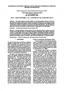
Figure 1: Dual objective during iterations using ve Figure 2: Optimal storage energy content and Ladierent methods to calculate []n+1. grangian multipliers. has failed to increase in ve iterations. The initial [i ]n, i = 1; :::; I , is set at 0:1. In practice, it should be rather easy to get the correct size of the initial multiplier value since i can be interpreted as the marginal value of stored heat in time interval i. Here i = 0:1 means 100 Swedish kroner (SEK) per produced MWh. Notice that Method 3 and Method 5 are using the optimal dual value  = 1084:236 in the calculation of  in (20). In real applications,  is unknown. It is in fact  we are searching for. To get a fair comparison, every calculated ([]n+1) in Step 5 is depicted, see Figure 1, or equivalently, n in Step 7 is updated every time a new ([]n+1) is computed. The calculations are interrupted after 100 iterations. We see that the performances are entirely dierent. Due to the use of a constant  in Method 1, we get the characteristic zig-zagging. In Method 2, a new subgradient s is calculated only when ([]n+1) is improved, leading to small , and thereby small improvements of ([]n+1) before []n is updated. Method 4 exploits the same idea, but does not treat the dierent i independently. As illustrated by Figure 1, this gives much more robust results. During the one hundred calculations, it is only Method 4 and Method 5 that approach the optimal dual value  = 1084:236 rapidly. Our test case clearly shows that Method 4, or its improved version, Method 5, are the superior methods. Hence, the exploitation of the interdependencies between the optimal dual values, see the next section, is clearly benecial for the construction of ecient computational methods.

that the storage energy content ei;S is not on its bounds, i.e. ei;S < ei;S < ei;S , the marginalvalues of stored heat in time intervals i ? 1 and i must be equal. If they are not equal, it would be more economical to charge the storage in the time interval with lower marginal value, and discharge it in the time interval with higher marginal value. Taking into account the losses and storage bounds will give the conditions already stated in (17). In particular (17) implies that when the storage is on the upper bound ei;S (lower bound ei;S ), then i?1  i (1 ? li;S ) (i?1  i (1 ? li;S )). This is the observation behind the Backwards Sequential Projection Algorithm of Section 3. We will now verify this on the test case used in Section 5. In Figure 2, the (optimal) ei;S and i resulting from the algorithm using Method 4 are shown. In time interval 7, the storage energy content is at its lower bound, and in time interval 19 it is at its upper bound. This has a rather trivial physical explanation. The plant includes one cogeneration unit operating in back-pressure mode, i.e. the produced heat and power are proportional. Increasing the electricity production thus leads to a higher production of heat (and vice versa). A high electricity price opens up the prospect of making prots at the electricity market, i.e. when the price is high, it is desirable to produce as much electrical power as possible. As a consequence, the total heat production increases, and if it exceeds the heat demand, the solution is to charge the storage. This is the situation during the time intervals 7 to 18. Equivalently, it is cheap to produce heat during this period, i.e. the marginal value of stored heat in the time intervals 7 to 18 is low (in our case, 109 SEK/MWh or 1000i, i = 7; :::; 18). In the time intervals 7, 8, 17 and 18, the total heat production 6 INTERPRETATIONS is limited by the maximum storage charge capacity qi;S The multiplier i can be interpreted as the marginal (the slope of ei;S in Figure 2). value of stored heat in time interval i. Assuming that The interpretation and the relation between the mul0 = 0 in (6), and tipliers, i?1 = i (1 ? li;S ) when ei;S < ei;S < ei;S , there are no losses, i.e. li;S = 0 and li;S 6

make it possible to separate the problem into independent subproblems. Once the time intervals where either ei;S = ei;S or ei;S = ei;S are detected (in our case, in less than ten iterations), ei;S can be xed at respective boundary (in our case, e7;S = e7;S and e19;S = e19;S ), leading to a decomposition of the problem. In our case, this is equivalent to solving three independent subproblems; one for the time intervals 1 to 6, one for the time intervals 7 to 18 and one for the time intervals 19 to 24, each interval having a unique marginal value of stored heat. However, this potential improvement in computational eciency was not exploited here. There are also clear interpretations of the relations between the marginal values of stored heat and the marginal production costs. Thus, if (4) is not binding for unit k, the marginal production cost is uniquely dened  + 1 , where q is the optimal production as 22i;k qi;k i;k i;k  +  1 = i . level. From (22) it is seen that 22i;k qi;k  i;k satisfy Assuming that i;S = 0, and the optimal qi;S  < qi;S , then i = i, cf. (23). Therefore, qi;S < qi;S in this situation, the marginal cost of production, i , is equal to the marginal value of stored heat, i . If further i?1 = i (1 ? li;S ), then i?1 = i (1 ? li;S ), i.e. the marginal production costs in the two periods deviate only in accordance with the storage loss. If (8) is binding, then possibly i 6= i . If i;S > 0 and (8) is not  + i ? i = 0, i.e. the marginal cost binding, 2i;S qi;S of production and the marginal value of stored heat deviate by an amount proportional to the cost of the heat storage. To sum up, it is seen that the dual variables permit detailed interpretation of the relation between production and storage costs and between consecutive time intervals. Further, this provides the basis for the ecient algorithms presented in Section 3.

The distinguishing feature is the exploitation of the observation that there must be specic numerical relations between the optimal Lagrangian multipliers. The paper also shows how these relations may be motivated by economic interpretations of the structure of the optimal solution. Thus, the paper exemplies the benet that may be achieved by considering the derivation of optimality conditions, their interpretations and the algorithm construction as integrated activities.

7 CONCLUSIONS

Systems, Vol. 18, No. 4, pp. 207 - 214, 1996. [6] Sturla Sæther and Hans F. Ravn, Simulations of

REFERENCES [1] Erik Dotzauer, Algorithms for Short-Term Production-Planning of Cogeneration Plants, Licentiate Thesis No. 644, ISBN 91-7219-033-7, ISSN 0280-7971, Division of Optimization, Department of Mathematics, Linköping University, Linköping, Sweden, 1997. [2] Stefan Feltenmark, On Optimization of Power Production, PhD Thesis, TRITA-MAT 97-OS1, ISSN 0348-405X, ISRN KTH/OPT SYST/DA97/1SE, Department of Mathematics, Royal Institute of Technology, Stockholm, Sweden, 1997. [3] K. Ito , R. Yokoyamaand T. Shiba, Optimal Operation of a Diesel Engine Cogeneration Plant Including a Heat Storage Tank, Journal of Engineering for

Gas Turbines and Power, 114:687-694, 1992. [4] Hans F. Ravn and Jens M. Rygaard, Optimal Scheduling of Coproduction with a Storage, Eng. Opt., 22:267-281, 1994. [5] M. F. J. Bos, R. J. L. Beune and R. A. M. van Amerongen, On the incorporation of a heat storage device in Lagrangian Relaxation based algorithms for unit commitment, Electrical Power & Energy

The paper has treated an aspect of the operation of a cogeneration system, in particular one with a heat storage. This is a problem of increasing importance, since such systems are becoming more common due to their relatively high energy eciency and the importance of the resulting environmental advantages. Moreover, with liberalized markets and the associated increased focus on cost reduction, ecient operation is essential. It has been shown how a short-term (one day) operation problem may be formulated as an optimal unit commitment and an economic dispatch problem. For this problem, an ecient algorithm has been presented. The algorithm is based on Lagrangian relaxation of the time equation of the storage. Together with the costs and restrictions related to the unit commitment, this equation constitutes the time couplings. The solution structure is exploited to obtain an algorithm and it is shown in a case study that it clearly outperforms more straightforward Lagrangian approaches.

Combined Heat and Power Systems with Heat Storage, Proceedings, MEGASTOCK '97, June 18-21,

1997, Sapporo, Japan, Vol. 1, pp. 205 - 210. [7] Hans F. Ravn, Lagrangian Relaxation of an Optimal Control Problem, In Proceedings, First Nordic Meeting on Mathematical Programming, 103-114, IMSOR, Technical University of Denmark, 1990. [8] N. Z. Shor, Minimization Methods for NonDierentiable Functions, Springer-Verlag, 1985. [9] Sabur Sen and D. P. Kothari, Optimal thermal unit generating unit commitment: a review, Electrical Power and Energy Systems, Vol. 20, No. 7, pp. 443 - 451, 1998.

7