The problem of trajectory planning for high-speed ..... R(s). lR. lF. fRy. fRx. fF y. fF x Ï. xB. Fig. 6. A half-Car Model of a vehicle driving along a prescribed path.
Optimal Velocity Profile Generation for given Acceleration Limits; The Half-Car Model Case E. Velenis∗ and P. Tsiotras∗
∗ Georgia
Institute of Technology School of Aerospace Engineering, Atlanta, GA, USA {efstathios velenis, p.tsiotras}@ae.gatech.edu
Abstract— A method to generate on-line optimal acceleration/deceleration and attitude profiles for a half-car model in high-speed cornering is presented. The methodology is an extension of [1] where a point-mass model of the vehicle was used. The acceleration envelope of the vehicle (GGdiagram) from the locus of the front and rear tire forces is used for selecting the optimal control inputs. A stable implementation of the algorithm for a path of increasing radius is also presented.
I. I NTRODUCTION The problem of trajectory planning for high-speed autonomous vehicles is typically dealt with in the literature by means of numerical optimization. Several results have been recently published [2], [3], [4], [5] for highspeed ground vehicles to demonstrate that these numerical techniques allow the incorporation of accurate, high-order dynamical models in the optimization process producing realistic results. In fact, the optimal solutions generated by these optimizers are comparable to experimental results generated by expert-race drivers [5]. On the other hand, these numerical optimization approaches are computationally costly and cannot incorporate unpredictably changing environments (consequently, they may not be suitable for real-time implementation). An alternative approach is proposed in this work. With the aim of minimizing the computational cost, we examine the possibility of solving the problem of trajectory planning, (or at least part of the problem) analytically. Our approach is to separate the geometric and dynamic parts of the design of the optimal trajectory. We assume that the geometric characteristics of the path to be followed are given, for instance by means of a prior numerical optimization. For example, the path to be followed could be a path of minimum distance, or a path of minimum average curvature, or a path of minimum combined cost. Since the dynamics of the vehicle are not included in this first step of the optimization process we expect minimal computational cost. The part of the dynamic trajectory design consists of the calculation of the optimal velocity profile through the prescribed path, given the dynamics of the vehicle. A semi-analytical method that provides an intuitively optimal velocity profile is proposed in [6], [7]. Formal proof of optimality of this semi-analytical methodology is provided in [1] as well as a study of several uncontrollable cases neglected in [6], [7]. Finally, in order for the trajectory planning scheme to be safely applied on-line
a receding horizon implementation of the optimization methodology has been presented in [8] to incorporate unpredictably changing environments. In this work the methodology of [6], [7] and [1] to generate the optimal velocity profile on a prescribed path for the minimum time travel of a vehicle with given acceleration limits is extended to a half-car model. This extension provides the attitude information missing from [6], [7] and [1]. Additional challenges include the determination of the acceleration envelope at the C.G. of the vehicle (GG-diagram), which is changing with the vehicle’s operating condition, as well as the stability of the yaw dynamics. In the following, the methodology of [6], [7] and [1] is reviewed. A half-car model with nonlinear tire friction characteristics is used to calculate the acceleration envelope of the vehicle for any operating condition. An extension of the optimal control strategy of [1] is then proposed using the dynamics of the half-car model. Numerical simulations reveal that the stability of the yaw dynamics needs to be taken into consideration. II. O PTIMAL V ELOCITY P ROFILE FOR A P OINT-M ASS V EHICLE Consider a vehicle of mass m travelling through a prescribed path, given the acceleration limits and fixed boundary conditions, i.e. fixed initial and final position and velocity. The velocity profile through the path for minimum time travel is investigated. The path is described by the radius at each point of the path as a function of the path length coordinate s, R(s) (Fig. 1) or, equivalently, by the curvature k(s). The cartesian coordinates of any point on the path can be calculated using a standard transformation [4], [8]. The equations of motion are given ftmax R(s)
B
fnmax m
A s Fig. 1. The point mass m travels along the prescribed path R(s), given maximum acceleration limits, in minimum time.
70
60
(1)
where, ft is the force tangential to the path and fn is the force normal to the path. Since we assume that the path is followed exactly by the vehicle, the normal force fn is given by (1). The control input is ft . We also consider given acceleration limits, which result in the following control constraint: �2 � �2 � fn ft + − 1 ≤ 0, (2) ftmax fnmax where ftmax is the maximum longitudinal and fnmax the maximum lateral forces repsectively. Introducing a new control variable u, the control constraint may be rewritten as follows � �2 � �2 � ds m ftmax 2 (3) ft = u (ftmax ) − R fnmax dt where u ∈ [−1, +1]. Assuming that the trajectory remains inside a region where controllability is maintained and the dynamics are well defined, it is formally proven in [1] that for minimum time travel the maximum available force is used at all times, i.e. the optimal control consists of sub-arcs of full acceleration (u = +1) or full deceleration (u = −1). Note that there exists a critical velocity � � ds �� R max (4) = v = f critical n dt �critical m for which ft = 0. In this case fn = fnmax , that is, the total acceleration capacity of the vehicle is used to produce the required centripetal force, and subsequently, no available force remains for longitudinal acceleration/deceleration. Thus at v = vcritical loss of controllability ensues. In other words, vcritical is the maximum allowable velocity at each point of the path. The reader is referred to [1] for detailed discussion. The optimal velocity profile in [1] is constructed as follows. • First, the points of local minima of the path radius and the areas of constant radius are identified. For a path with radius profile as in Fig. 2, the points of interest are points P1 , P2 and P5 of local minima of the radius and the interval between points P3 and P4 of constant radius. • The optimal velocity profile subject to free boundary condition for each of the subarcs containing the points of interest is then calculated. For the subarcs containing a unique point of local minimum radius, this profile consists of full deceleration (u = −1) before, and full acceleration (u = +1) after each of the local minima. The velocity at each of the local minima is equal to vcritical for the given minimum radius. In Fig. 3 the characteristic (i) corresponds to point P1 , characteristic (ii) corresponds to point P2 and characteristic (iv) to point P5 . For the intervals of constant radius, this profile
P
1
50
40
R (m)
� �2 m ds d2 s dt = fn , m 2 = ft , dt R(s)
P3
P
4
30
P
5
20
P2
10
p2
p
1
p3
0 0
p5
p4 45
90
s (m)
Fig. 2.
A “general case” radius profile path
8
(i) 7
6
ds/dt (m/sec)
by
(iii)
5
(iv) 4
(ii)
3
2
1
p1 0 0
p
2
p3
p
4
45
p5 90
s (m)
Fig. 3. The unconstrained problem solutions for constant radius and min{R} sub-arcs.
consists of constant velocity as close (but not equal) to vcritical as possible. In Fig. 3 the characteristic (iii) corresponds to the interval between points P3 and P4 . • Given the boundary conditions, for example, the initial point A and the final point B in Fig. 4, we construct the characteristic of full acceleration (u = +1) from the initial point (characteristic (I) in Fig. 4) and the characteristic of full deceleration (u = −1) towards the final point (characteristic (II) in Fig. 4). • The optimal velocity at each point of the path is the minimum of all the above characteristics at that certain point. For the example under consideration, this approach yields v ∗ (s) = min{v k (s)} , k = i, ii, iii, iv, I, II, with v k (s) being the velocity profile corresponding to the k characteristic (solid line in Fig. 4). This methodology has been used to generate the optimal velocity profile for an F1 circuit, given the acceleration limits of a typical F1 race car, and to compare to results achieved by expert F1 race drivers [8]. The results are shown in Fig. 5. III. E XTENSION TO A H ALF -C AR M ODEL In this section we extend the methodology described in the previous section to a half-car model in order to derive the missing attitude information of the vehicle’s
8 (i) 7 A
(I) 6
(iii)
ds/dt (m/sec)
5
R(s)
(iv) 4
(II)
(ii)
B
yI
3
v
β 1
0
fRy 0
10
20
30
40
50
60
70
80
fF x
xB
ψ
yB
xI
2
fF y
C.G.
fRx
φ
�F
90
s (m)
Fig. 4.
Optimal velocity profile for the “general case” path.
350
350
300
300
250
s
250
Speed (km/h)
200 Speed km ( /h)
�R
150
100
200
Fig. 6. A half-Car Model of a vehicle driving along a prescribed path R(s).
150
100
50
50
Lap1 Lap2 Lap3 0 0
1000
2000
3000 Lap Distance (m)
(a)
4000
5000
6000
0
0
1000
2000
3000 4000 Lap Distance (m)
5000
6000
(b)
Fig. 5. Velocity profiles through the Silverstone circuit: experimental (a) from [9], computed optimal (b).
orientation. The equations of motion of a half-car model along a prescribed path R(s) as in Fig. 6 are given below. m¨ x =
(fF x + fRx ) cos ψ − (fF y + fRy ) sin ψ, (5)
m¨ y = (fF x + fRx ) sin ψ + (fF y + fRy ) cos ψ, (6) (7) Iz ψ¨ = fF y �F − fRy �R . The self-aligning torque Mz is neglected, as it is typically done in the literature [3], [4], [5]. In the above equations m is the vehicle’s mass, Iz is the polar moment of inertia of the vehicle, and x and y are the cartesian coordinates of the C.G. in the inertial frame of reference. ψ is the yaw angle of the vehicle and by fji (j = x, y, i = F, R) we denote the friction forces of the front and rear wheels, respectively, along the longitudinal and lateral body�axes. Equations (1) will also be used, with ds/dt = v = x˙ 2 + y˙ 2 , and ft , fn the components of the resultant force, due to front and rear wheel friction, along the tangential and normal directions of travel respectively. Define the path angle φ and the vehicle slip angle β as follows (see Fig. 6): � � y˙ φ = arctan , β = φ − ψ. (8) x˙ The tire friction forces are calculated using Pacejka’s “Magic Formula” model [10] as follows. sij tire = − Fi (i = F, R and j = x, y), (9) fij si tire where, fij (i = F, R and j = x, y) are the components of the front and rear wheel friction forces along the
longitudinal and lateral tire axes respectively, six is the longitudinal and siy is the lateral slip of the i wheel. tire should not be confused with the The components fij components fij of the same forces along the longitudinal and lateral body axes, used in equations (5)-(7). The total friction force of the front and rear wheel, Fi (i = F, R), is computed using Fi = Fiz D sin(Catan(Bsi )) (i = F, R),
(10)
where Fiz (i = F, R) is the vertical load at the front and rear axle, respectively, and the total slip si (i = F, R) is computed as si = s2ix + s2iy with i = F, R. (11) The friction force of each wheel lies within a circle of radius equal to the maximum friction force fimax (i = F, R), for smax , provided by (10) as in Fig. 7. i We assume that we can control the front and rear longitudinal slip six , (i = F, R) of the front and rear wheel independently, as well as the steering angle δ of the front wheel. Using the standard definition of longitudinal slip [10] we choose six ∈ [−1, +1]. The expressions for the lateral slip of the front and rear wheels are given below: sRy
=
sF y
=
˙ R v sin β − ψ� , v cos β ˙ F cos δ v sin(β − δ) + ψ� . ˙ F sin δ v cos(β − δ) + ψ�
(12) (13)
The rear lateral slip sRy is completely determined by the states of the system, i.e., sRy is fixed for a given ˙ Thus, for a operating condition of the vehicle (v, β, ψ). given operating condition of the vehicle, and assuming that we can control the rear longitudinal slip, the rear friction force lies on a characteristic curve determined by the lateral slip sRy as in Fig. 8.
2000
1
(smax, fmax) i
1800
i
v = 30m/sec β = 10deg dψ/dt = 0.1 rad/sec
0.8
0.6
1400
0.4 front wheel lateral slip s
Total Tire Force (N)
Fy
1600
1200
1000
800
0.2
0
−0.2
600
−0.4
400
−0.6
200
−0.8
0
0
0.1
0.2
0.3
0.4
0.5 0.6 Combined Slip
0.7
0.8
0.9
−1 −60
1
Fig. 7. Total friction force of the ith wheel with respect to the combined slip as given by the Magic Formula
v = 20m/sec β = −25deg dψ/dt = 0.5 rad/sec
−40
−20
0 steering angle δ (deg)
20
40
60
Fig. 9. Front lateral slip with respect to steering angle for given operating condition of the vehicle.
2000 s = −0.21 iy
1500
1000
siy = −0.6
fiy (N)
500 siy = 0 0 s = 0.01 iy
−500
−1000
siy = 0.05 siy = 0.15
−1500
−2000 −2500
−2000
−1500
−1000
−500
0 fix (N)
500
1000
1500
2000
2500
Fig. 8. Front and rear tire friction characteristic curves for fixed lateral slip siy (i = F, R) and longitudinal slip six ∈ [−1, +1] (i = F, R).
calculate the necessary centripetal force fn from (1) such that the vehicle follows the path. We can also determine the tangential and normal directions to the path with respect to the orientation of the vehicle (these are denoted by t and n respectively in Fig. 10). The calculated fn lies along the n direction and may be produced by only two possible total forces ftot on the GG-diagram. One of the two ftot forces produces an accelerating tangential force ft , which corresponds to the u = +1 strategy of Section II, and the other produces a braking force that corresponds to the u = −1 strategy. As already mentioned, each force ftot on the GG-diagram is associated uniquely to a pair of front and rear friction forces, thus enabling us to integrate equations (5)-(7).
3500 3000
n
GG−diagram
2500
fn
2000
ftot (accel.) ftot (braking)
1500 fy (N)
The front lateral slip sF y , however, depends on the steering angle δ, which is one of the control variables. Figure 9 demonstrates that for any vehicle operating condition we may generate any front wheel lateral slip, max sF y ∈ [−smax F , +sF ] using a steering angle δ within a realistic range of δ ∈ [−π/4, +π/4]. In Fig. 8 it is also demonstrated that the whole friction circle including its interior can be constructed by characteristics of + smax sF y ∈ [−smax F F ]. Thus, we conclude that given any operating condition of the vehicle, and assuming that we can control the front longitudinal slip and steering angle, the front friction force may be chosen anywhere inside the friction circle. The resultant force at the C.G. of the vehicle is found by adding the front and rear friction forces. The resultant force envelope (GG-diagram) is constructed, for each operating condition of the vehicle, by adding the front friction circle to the rear wheel friction characteristic, as in Fig. 10. Any point on the force envelope is associated with a unique pair of front and rear tire friction forces. An extension of the optimal control strategy described in Section II becomes evident. Given an operating condition of the vehicle (velocity components x˙ and y, ˙ orientation ˙ and the geometry of the path, we can ψ, yaw rate ψ)
1000 t
500
ft (accel.)
0 rear wheel friction characteristic
−500 f (braking) t
−1000
xB
front wheel friction circle
−1500 −3000
−2000
−1000
0 f (N)
1000
2000
3000
x
Fig. 10.
GG-diagram for a given operating condition of the vehicle.
In the next section we present an extension of the optimal velocity profile generation for a path with a point of minimum radius, subject to free boundary conditions using a half-car model of the vehicle. For brevity, we omit the constant radius path case. Since there is no acceleration or deceleration, the GG-diagram would remain constant and the optimal strategy would be a steady-state corner of constant velocity (vcritical ) and slip angle.
35
IV. N UMERICAL S IMULATION 30
5 t = 2.5 sec 0
−5
y(m)
t = 1 sec
t = 4 sec
−10
−15
t=0
t = 5 sec
−20
−25 −20
−15
−10
−5
0 x(m)
5
10
15
20
Fig. 11. Snapshots along a path with a point of minimum radius at (x, y) = (0, 0)
44
42
40
25
20 β (deg)
Consider a path with a point of minimum radius at point (x0 , y0 ) = (0, 0), as in Fig. 11. The path for this example is described by R(s) = 0.5s − 10 m before point (x0 , y0 ) (where we set s = 0) and R(s) = −0.5s − 10 m after that point. The strategy described in Section II dictates that the vehicle should be travelling at point (x0 , y0 ) with vcritical . The control should be the equivalent to u = −1 before, and u = +1 after the point x0 , y0 . The initial condition at (x0 , y0 ) is calculated numerically such that the total force of the GG-diagram is along the normal direction and equal to the sum of the maximum forces fimax (i = F, R). Forward integration for 2.5sec with u = +1 and backward integration for another 2.5sec with u = −1 from the calculated initial condition results in the trajectory of Fig. 11 and the velocity profile of Fig. 12. In Fig. 13 the vehicle slip angle β with time is shown. We observe
15
10
5
0
0
0.5
Fig. 13.
1
1.5
2
2.5 t (sec)
3
3.5
4
4.5
5
Vehicle slip angle β with time.
that follows we propose an alternative strategy in order to avoid this instability in the yaw dynamics. V. S TABILITY OF YAW DYNAMICS Research on stability of passenger vehicle yaw dynamics has led to the development of systems like the Electronic Stability Program (ESP) [11] that uses individual wheel braking in order to generate stabilizing yaw moments in critical cases where the vehicle operates close to an estimated stability margin. In practice this margin is characterized by the vehicle slip angle [11]. A more careful approach shows that the stability margin depends on the combination of the vehicle slip angle and its rate of change [12]. However, no formal, closedform characterization of the stability margin of the yaw dynamics is available in the literature. In this section we propose a simple approach to implement the velocity profile generation scheme, described in the previous sections, avoiding yaw instability. As in the ESP system, we use the vehicle slip angle β information to detect whether the vehicle tends to an unstable operating condition. When a critical value of β is reached, the u = ±1 strategy, described in Section IV, is aborted. Instead, the total friction force from both the front and rear tires is generated along the normal direction, contributing only to the centripetal force (Fig 14). That is,
v (km/h)
38
FF + FR = fn when β ≥ βcritical .
36
34
32
30
28
0
0.5
1
1.5
2
2.5 t (sec)
3
3.5
4
4.5
5
Fig. 12. Velocity profile along the path with a point of minimum radius.
that straightforward application of the strategy of Section II may result in instability of the yaw dynamics. This is due to the fact that the vehicle slip increases at a fast rate (Fig. 13) resulting in increasing magnitude of the rear lateral slip and a shrinking GG-diagram (observe the characteristic of siy = −0.6 in Fig. 8). We thus reach a point where the fn required for the vehicle to follow the path is outside the available force envelope. In the section
(14)
The rear wheel force FR is chosen to be along the n direction. Given the operating condition of the vehicle and thus the rear wheel friction characteristic, the choice of the rear wheel force is unique. The front wheel friction force FF is chosen also uniquely, such that (14) holds. This choice of front and rear friction forces results in zero acceleration force along the t direction, and in a stabilizing yaw moment. The fact that there is no acceleration also helps in decreasing the demand for centripetal force. The control logic (14) is applied successfully to the increasing radius subarc of the path of the previous section (Fig. 15). The velocity profile does not increase monotonically anymore (that is after t = 2.5 sec), but it is interrupted by intervals of zero acceleration (Fig. 16), while the vehicle slip angle remains bounded (Fig. 17). For this preliminary approach to a stable implementation
75
70
65
n
f =f +f n
F
R
60
v (km/h)
55
f
R
50
fy
45
t
fn
40
35
fF
30
25
0
2
4
6
8
10
12
14
t (sec)
Fig. 16. Stable implementation of the velocity profile generation scheme; velocity profile. fx 18
Fig. 14. When the vehicle slip angle increases the front and rear wheels contribute only to the centripetal force.
16
14
12
10 β (deg)
of the “velocity profile generator” using a half-car model we chose the switching function (βcritical ) to be constant. Its value of 10 deg was chosen by trial and error. A more sophisticated approach would be to choose a velocitydependent value, that is, βcritical = βcritical (v). This choice is currently under investigation.
8
6
4
2
0
−2
0
2
4
6
8
10
12
14
t (sec)
10
Fig. 17. Stable implementation of the velocity profile generation scheme; vehicle slip angle with time.
t = 2.5 sec
0 t = 12.5 sec
−10
y (m)
t = 5 sec
−20
t = 0 sec
−30 t = 10 sec
−40
−50
−60
−70
−60
−50
−40
−30 x (m)
−20
−10
0
10
Fig. 15. Stable implementation of the velocity profile generation scheme; trajectory.
VI. C ONCLUSIONS In this work we have presented a semi-analytical method to generate velocity profiles for “fast” path following using a half-car model. Some preliminary work on stable implementation of the methodology has been discussed. Immediate extensions of this work may include, calculation of the “real” control inputs (wheel torques and steering angle) using the known slip quantities and the wheel dynamics, comparison of the velocity profile generated with numerical optimization solutions, and a formalized proof of yaw stability. R EFERENCES [1] E. Velenis and P. Tsiotras, “Optimal velocity profile generation for given acceleration limits: Theoretical analysis,” in Proceedings of the American Control Conference, June 8 - 10 2005. Portland, OR (to appear).
[2] T. Fujioka and M. Kato, “Numerical analysis of minimum-time cornering,” in Proceedings of AVEC 1994, November 24-28 1994. Tsukuba, Japan. [3] J. Hendrikx, T. Meijlink, and R. Kriens, “Application of optimal control theory to inverse simulation of car handling,” Vehicle System Dynamics, vol. 26, pp. 449–461, 1996. [4] D. Casanova, R. S. Sharp, and P. Symonds, “Minimum time manoeuvring: The significance of yaw inertia,” Vehicle System Dynamics, vol. 34, pp. 77–115, 2000. [5] D. Casanova, R. S. Sharp, and P. Symonds, “On minimum time optimisation of formula one cars: The influence of vehicle mass,” in Proceedings of AVEC 2000, August 22-24 2000. Ann-Arbor, MI. [6] M. Gadola, D. Vetturi, D. Cambiaghi, and L. Manzo, “A tool for lap time simulation,” in Proceedings of SAE Motorsport Engineering Conference and Exposition, 1996. Dearborn, MI. [7] M. Lepetic, G. Klancar, I. Skrjanc, D. Matko, and B. Potocnic, “Time optimal path planning considering acceleration limits,” Robotics and Autonomous Systems, vol. 45, pp. 199–210, 2003. [8] E. Velenis and P. Tsiotras, “Optimal velocity profile generation for given acceleration limits: Receding horizon implementation,” in Proceedings of the American Control Conference, June 8 - 10 2005. Portland, OR (to appear). [9] Anonymous, “RT3000 inertial and GPS measurement system, report from Silverstone F1 test,” Technical Report, Oxford Technical Solutions, Oxfordshire, UK, 2002. [10] E. Bakker, L. Nyborg, and H. Pacejka, “Tyre modelling for use in vehicle dynamics studies,” SAE paper # 870421, 1987. [11] A. T. van Zanten, R. Erhardt, and G. Landesfeind, K. Pfaff, “Vehicle stabilization by the vehicle dynamics control system ESP,” in IFAC Mechatronic Systems, (Darmstadt, Germany), pp. 95–102, 2000. [12] K. Koibuchi, M. Yamammoto, Y. Fukada, and S. Inagaki, “Vehicle stability control in limit cornering by active brake,” SAE Special Publications, Investigations and Analysis in Vehicle Dynamics and Simulation, no. 1141, pp. 163–173, 1996.