Ashby Road, Loughborough, LE11 3TU. 2 Institute of Science and Technology,. University of Keele, Thornburrow Drive, Hartshill, Stoke-on-Trent ST4 7QB.
Report on a problem studied at the UK Mathematics-in-Medicine Study Group Nottingham 2006 < http://www.maths-in-medicine.org/uk/2006/tissue-engineering/ >
Optimisation of Fluid Distribution inside a Porous Construct Clare Bailey1 , Richard Booth4 , Sarah Cartmell2 , Louise Parsons Chini3 , Linda Cummings3 , Rosemary Dyson4 , Vipin Michael2 , Shailesh Naire3 , Sevil Payvandi6 , Zimei Rong5 , Sarah Waters3 , Robert Whittaker3 & Hannah Woollard3 . 1
Department of Civil and Building Engineering, Loughborough University, Ashby Road, Loughborough, LE11 3TU. 2 Institute of Science and Technology, University of Keele, Thornburrow Drive, Hartshill, Stoke-on-Trent ST4 7QB. 3 School of Mathematical Sciences, University of Nottingham, Nottingham, NG7 2RD. 4 Mathematical Institute, University of Oxford, 24-29 St Giles’, Oxford, OX1 3LB. 5 Interdisciplinary Research Centre in Biomedical Materials, Queen Mary University of London, Mile End Road, London, E1 4NS. 6 Department of Bioengineering, Imperial College London, South Kensington Campus London, SW7 2AZ.
1
Introduction
Bone tissue is an important part of the human body, providing necessary support, storage of calcium and production of immune protection cells. Bone can be damaged either by disease or trauma. Each year in the United Kingdom, over 1800 people are diagnosed with a bone or connective tissue cancer [3]. Osteoporosis is a disease posing a huge threat affecting 55% of individuals over the age of 50 years. In the United States, ten million individuals are estimated to already have the disease, and almost 34 million more are estimated to have low bone mass, placing them at increased risk for osteoporosis [6]. Bone fractures are experienced by about 6.8 million of the US population every year. Cartilage provides the necessary lubrication and shock absorbance that is needed when joints move together. Cartilage degeneration occurs in patients suffering from arthritis. Twenty million people suffer from some sort of arthritis in the UK. Therefore, the impact on helping prevent the onset of this debilitating disease is huge. Cartilage can also be damaged by trauma. If the cartilage is damaged superficially (and the damage does not penetrate bone) then repair is poor. Cartilage cells do not proliferate well in vivo and as such repair suffers. When the damage penetrates through the cartilage tissue reaching the underlying bone, delivery of progenitor cells occurs (from bone marrow) and fibrous cartilage formation occurs. This fibrous cartilage is of a poorer quality than the original cartilage and can often lead to the 1
(a)
(b)
Figure 1: (a) MicroCT and photographs of the porous hydroxyapatite scaffolds provided by Dr Jon Gittings and Dr Irene Turner at Bath University; (b) Schematic of position of PLGA fibres to be inserted into scaffold. onset of osteoarthritis. Often the damage to the bone and cartilage is treated with permanent implants (such as total knee/hip replacements) to replace the tissue. However, these implants have limitations, mainly with regard to their longevity. Tissue engineering is an emerging therapy that offers a new solution to patients suffering from the kind of diseases outlined above. This therapy utilizes cells that are derived from sources such as the patient’s own bone (a section of bone such as the rib that is not damaged) or from their bone marrow. These cells are isolated in the laboratory and grown so that they multiply in number. Then they are placed onto a degradable material, called a scaffold, that has mechanical and chemical properties appropriate to the piece of bone that it is replacing. The cells plus the scaffold are then grown in a container called a bioreactor. This bioreactor is necessary as it provides the correct environment that is needed for the cells to grow well and produce bony matrix. Nutrient delivery and waste disposal is of vital importance to each of the cells that reside within the scaffold. The larger the piece of bone or cartilage that is attempted to be grown, the more challenging the nutrient and waste diffusion dynamics. Very little research has been directed at designing a bioreactor to provide optimum conditions for cultivating bone and cartilage together. Current strategies to improve the nutrient delivery to, and waste removal from, cells seeded onto a 3D scaffold take advantage of the 3D scaffold morphology. Typically, 3D scaffolds are of a high porosity (70–90%), with pore sizes ranging in size from 250 µm to 600 µm. The nutrients are delivered to the cells via a liquid called culture medium. The nutrients that the cells need are many and include oxygen, glucose, ascorbic acid (vitamin C) and various 2
salts and proteins. The cells produce waste such as lactate and carbon dioxide (which builds up in the local area and lowers the pH of the surrounding medium, which is destructive to the cell). To assist in the delivery and removal of these products, the culture media is often mixed around or perfused directly through the 3D scaffold to prevent stagnant regions. For small samples of tissue (such as 4 mm height × 10 mm diameter cylindrical specimens) these methods have been shown to be successful in comparison to static culture. In static culture, the cells in the centre of such samples die and only the cells at the periphery of the construct prevail. With direct perfusion and mixing techniques, a problem arises when the tissue sample size is scaled up. Standard mixing techniques (i.e. forcing the flow through the sample by some exterior means) alone will not be satisfactory in delivering media throughout a larger scaffold. If the centre of the construct is to receive adequate medium delivery, then the exterior of the construct suffers by receiving too much shear stress from the flowing fluid and cells begin to die. When a large scaffold undergoes perfusion alone, a risk is incurred of developing stagnant regions as it becomes increasingly difficult to reach all areas as size increases. Because of this limitation, we have designed a new approach to deliver nutrients to cells seeded in the centre of large constructs (we consider a large construct in tissue engineering terms to be 15 mm diameter × 16 mm height, consisting of 10 mm bone and 6 mm cartilage). In addition to perfusing medium through the scaffold in a conventional manner, two porous degradable polyglycolic acid (PLGA) fibres (manufactured by Dr Marianne Ellis and Professor Julian Chaudhuri, Bath University), each of 1 mm outer diameter, are incorporated into the scaffold system. Through the porous walls of these fibres, extra culture medium is perfused (not necessarily at the same rate as the full scaffold perfusion) in order to administer nutrients directly, and remove waste from cells, in the centre of these constructs. The porous hydroxyapatite scaffold used in this system is created by Dr Irene Turner and Dr Jon Gittings from the University of Bath (see figures 1a,b). The design of the capped porous hydroxyapatite scaffold mimics the physiological set up of porous trabecular bone having a cortical ‘cap’ as it meets the cartilage layer in an articulating joint. The scaffold morphology was created with the hypothesis that it would be beneficial to have a solid top (cap) to the porous scaffold to restrict mixing of the different media compositions in the bioreactor for the cartilage and bone culture conditions and therefore produce functional and separate tissue types. The outline of the novel bioreactor design is shown in figures 2 and 3, with dimensions and other properties given in table 1. 3
Figure 2: Cross-sections of the bioreactor, showing the positions of the inflow and outflow pipes and the two porous fibres.
4
Quantity Internal radius of chamber Internal height of bone section Internal height of cartilage section External radius of porous fibres Internal radius of porous fibres Porosity of scaffold Permeability of scaffold † Permeability of fibre wall Viscosity of culture medium Typical inlet volume flux
Symbol R∗ 2L∗ 2L0∗ b∗w b∗c φ k∗ kw∗ µ∗ Q∗+
Typical Value 7.5 × 10⁻³ m 10 × 10−3 m 6 × 10⁻³ m 0.5 × 10⁻³ m 0.17 × 10⁻³ m 0.8 10−10 –10−11 m2 †† 7.02 × 10⁻⁴ kg m−1 s−1 10−8 m3 s−1
Table 1: Dimensions and typical physical properties of the new bioreactor setup. † Permeability data was not directly available, but see §4.2 for a method of estimation. †† experimental measurement unavailable. The main novel features of the system are: 1. It is the first design to allow dynamic cultivation and mechanical stimulation to osteochondral tissue engineered constructs. 2. It incorporates a novel design of culture media administration throughout the bone section of the construct: both direct media perfusion and media delivery via two permeable fibres that run horizontally through the bone construct. 3. It allows the culture of larger tissue constructs than previously attempted (15 mm diameter × 16 mm height cylinders). The following questions were posed: 1. What are the flow dynamics and approximate shear stresses experienced in different areas of the 3D scaffold due to fluid flow in the bone portion of the sample only? 2. What is the optimal inlet flow rate of the culture medium for full distribution of media throughout scaffold? 3. 2D experiments have shown that shear stresses of 5–15 dyne cm−2 are beneficial to bone cells, but higher or lower stresses inhibit growth. What constraints does this range impose?
5
Figure 3: Photographs of the actual bioreactor prototype, showing its modular construction. This report is structured as follows. In §2 we develop an idealised 3D Darcy-flow model for the bioreactor system outlined above, considering just the lower bone chamber for simplicity. This model accounts explicitly for the presence of the hollow fibres, and identifies distinct flow regimes in which the flux out of the fibre is either constant along the fibre length (regime 6
1), varies linearly along the fibre length (regime 2), or is nonlinear (regime 3). Numerical solutions for the fluid flow throughout the porous scaffold in regime 1 are presented in §2.4. In §3 the specific scaffold pore geometry is considered (in contrast to the Darcy model of §2, which averages out the porescale geometry). Flow through 2D cross-sections of a scaffold with idealised pore geometry are considered, and a range of inlet and outlet pipe configurations are considered. In §4 we return to an averaged Darcy-flow description, and consider flow through 2D cross-sections of scaffolds with heterogeneous permeability. In §5 the problem of nutrient delivery and waste-product accumulation within the porous scaffold is considered briefly. Finally, in §6 we discuss the implications of the modelling results, and identify areas for future work.
2
Full 3D (idealised) model
The bone chamber of the bioreactor comprises a porous scaffold inside a circular cylindrical chamber of radius R∗ and height 2L∗ . Inflow and outflow pipes are situated on opposite sides, and two porous fibres run across the scaffold in the perpendicular direction, see figure 4. We consider the flow in the scaffold and the flow in the fibres as two separate problems, coupled by the continuity of pressure and the flux emitted through the fibre walls.
2.1
Flow in the outer scaffold
The scaffold pore geometry is of a random nature, with about 30 pores over its height, and the fluid velocities are low enough that the pore Reynolds number (based on a typical pore size of 0.5 mm) is small. We therefore model the scaffold as an isotropic porous medium, with a uniform permeability k ∗ (stars are used to denote dimensional quantities throughout). Although the growth of the bone will alter this permeability, such growth occurs over a period of weeks, which is much longer than the minutes required for fluid circulation. We therefore regard k ∗ as a constant. The Darcy velocity u∗ is related to the interstitial pressure p∗ by Darcy’s law [1]: u∗ = −
k∗ ∇p∗ , µ∗
(1)
where µ∗ is the dynamic viscosity of the fluid. Without loss of generality the zero point of the pressure is taken to be at the centre of the scaffold. Gravitational effects are either considered negligible, or absorbed into a modified pressure in the usual way. 7
R∗
x∗ = 0 y ∗ = −R∗ z∗ = 0
q (x )
Q∗+
y∗ = 0 z ∗ = −a∗
∗
y∗ = 0 z ∗ = a∗
∗
2a∗ = 2aR∗
−QQ∗+ x∗ = 0 y ∗ = R∗ z∗ = 0
2L∗ = 2`R∗
z∗ y∗ x∗
Figure 4: An overview of the bioreactor chamber, showing the positions of the inflow and outflow pipes (marked with dots), along with the two porous fibres (solid lines). We adopt a Cartesian coordinate system (x∗ , y ∗ , z ∗ ) aligned with the chamber, as shown in figure 4. We non-dimensionalize all lengths with the chamber radius R∗ , so in non-dimensional coordinates (x, y, z), the chamber occupies x2 + y 2 ≤ 1 , −` ≤ z ≤ ` , (2) where ` = L∗ /R∗ is the aspect ratio of the chamber. We non-dimensionalize fluxes with the flux at the inlet pipe, Q∗+ (which is typically set directly by the experimentalists), and define dimensionless velocities and pressures by u∗ =
Q∗+ u, R∗2
p∗ =
µ∗ Q∗+ p. k ∗ R∗
(3)
Darcy’s equation (1) then becomes u = −∇p .
(4)
For simplicity, we model the inflow and outflow as point sources of mass on the cylinder wall, with fluxes Q∗+ and −QQ∗+ , respectively, so that flux through outflow pipe . Q= (5) flux through inlet pipe Similarly, the thin fibres are assumed to provide line sources of mass, with spatially varying strength q ∗ (x∗ ) = q(x) Q∗+ /R∗ . 8
Conservation of mass relates ∇ · u to the various mass sources, and from (4) yields an equation for the dimensionless pressure: −∇2 p = 2 δ(x) δ(y + 1) δ(z) − 2Q δ(x) δ(y − 1) δ(z) � � + q(x) δ(y) δ(z − a) + δ(z + a) .
(6)
(Since the point sources are located on the domain boundary, the strengths are doubled in the above expression in order to obtain the correct fluxes inside the domain.) The boundary conditions for (6) arise from a no-penetration condition on the fluid flow across the boundaries. In terms of the pressure, we require ˆ · ∇p = 0 on z = ±` and on x2 + y 2 = 1 , n
(7)
ˆ is the unit normal to the boundary surface. where n The dimensionless flux per unit length q(x) from the fibres depends on the conditions applied at the fibre ends, and is considered in detail in §2.2 below. By global conservation of mass, and symmetry of the bioreactor geometry (so that the two fibres have identical flow) the dimensionless outlet flux is given by Z 1
q(x) dx .
Q=1+2
(8)
−1
If the flux per unit length q(x) from the fibres is known, (6)–(8) form a well-posed problem for the pressure p within the scaffold. We must now consider how to find q(x) using the conditions imposed at the ends of the fibres.
2.2
The flow in the fibres
The two porous fibres are modelled as circular cylinders of outer radius b∗w , with a hollow core of radius of b∗c . The walls are assumed to be made of a uniform isotropic porous medium with permeability kw∗ . Coordinates are x∗ in the axial direction and r ∗ = [y ∗ 2 + (z ∗ ± a∗ )2 ]1/2 in the radial direction, c.f. figure 4. Pressures are denoted by p∗ and velocities by u∗ = (u∗ , v ∗ ) with axial and radial components. We use subscripts c for the core and w for the walls, see figure 5. Boundary conditions are provided by continuity of pressure and radial mass flux at r ∗ = b∗w , together with imposed pressures P ∗ ∓ 12 ∆P ∗ at x∗ = ±R∗ . Written like this, ∆P ∗ is the pressure difference between the fibre ends, and P ∗ is a scale for the absolute pressure in the fibre (to be compared with p∗ ∼ µ∗ Q∗+ /k ∗ R∗ in the scaffold). 9
Outer Scaffold p ,u ������������������ �� � � � � � � � � � � � � � � � � � � � � � � � � � � � � � � � � � � � ������������������ �� � � � � � � � � � � � � � � � � � � � � � � � � � � � � � � � � � � � Fibre Wall ������������������ �� � � � � � � � � � � � � � � � � � � � � � � � � � � � � � � � � � � p , u ������������������ �� �� �� ������������������ �� ���� ���� ��(Darcy ���� ������flow,��������k ����) ����������������������������������� (Darcy flow, k ∗ )
r∗
∗
∗ w
∗ w
∗ w
p∗c , u∗c
Fibre Core 2b∗c
∗
(Stokes flow) ��� � � � ��� ��� �� � � � � � � �� �� ��������� ��������� ��������� ��������� ��������� ��������� ��������� ��������� ��������� ��������� ��������� ��������� ������ ��� ��� � � � � �� � � � � ���� � � � � � � � � � � � � � ��� ��� ��� ��� ��� � �� � �� � �� � �� � ������ ������ ������ ������ ������ ������ ������ ������ ������ ������ ������ ������ ���� ����� x∗
2b∗w
2R∗ Figure 5: The geometry of the porous-walled fibres, together with the variables used to describe the flow within them. A number of separations of scales help simplify the analysis of the flow in the fibre. The slenderness of the fibre (b∗c /R∗ � 1) and the relative impermeability of its wall (kw∗ � b∗2 c ) both help ensure predominantly axial flow in the core. If the pressure difference across the fibre wall is always large compared to the pressure difference along the fibre length (|P ∗ − µ∗ Q∗+ /k ∗ R∗ | � ∆P ∗ ), this helps ensure predominantly radial flow within the wall. Finally, a large pressure difference across the fibre wall compared with a typical pressure drop in the outer problem (P ∗ � µ∗ Q∗+ /k ∗ R∗ ; recall that we chose the zero of the pressure to be at the centre of the scaffold) means that the flow in the fibre can be solved without reference to the outer solution in the scaffold. Most of these assumptions are naturally satisfied in the physical system we set out to consider, and so minimal further restriction is required. Note that since the walls are fairly impermeable, a large transmural pressure difference P ∗ is necessary to get any significant outflow through the walls. 2.2.1
Non-dimensionalization
Assuming kw∗ /b∗2 c � 1, so that the tube lumen offers much less resistance to flow than the walls of the fibre, we will use the Stokes equations in the core and Darcy’s equation in the walls. We use non-dimensional axial and radial coordinates x∗ r∗ x= ∗, (9) r= ∗. R bc
10
` � λ 0.7 0.02 3
k ∗ /R∗2 10−4
kw∗ /b∗2 c †
α2 0.07
Table 2: Typical values of the various dimensionless parameters appearing in §2, computed from the values in table 1. †: require value of kw∗ . We also introduce two dimensionless parameters �=
b∗c �1 R∗
and
λ=
b∗w = O(1) . b∗c
(10)
The velocities and the pressures are non-dimensionalized in the natural way, by writing � � ∗ kw∗ P ∗ b∗2 ∆P ∗ c ∆P ∗ ∗ ∗ ∗ pc ; (11) vc = ∗ ∗ vc , uc = ∗ ∗ uc , pc = P 1 + µR µ bc P∗ u∗w =
kw∗ ∆P ∗ uw , µ∗ R ∗
vw∗ =
kw∗ P ∗ vw , µ∗ b∗c
p∗w = P ∗ pw .
(12)
We note the importance of the two pressure differences; the axial velocities are scaled on the pressure difference along the tube (∆P ∗ ),1 whereas the radial velocities are scaled on the pressure difference across the wall (P ∗ ). The axial mass flux in the core is denoted Q∗c and the radial flux per unit length in the wall is denoted qw∗ . Based on the corresponding velocity scales, we non-dimensionalize these fluxes as Q∗c =
2.2.2
∗ b∗4 c ∆P Qc , µ∗ R ∗
qw∗ =
kw∗ P ∗ qw . µ∗
(13)
Flow in the fibre core
The flow in the core is governed by the steady Navier–Stokes equations ρ∗ (u∗c · ∇∗ ) u∗c = −∇∗ p∗c + µ∗ ∇∗2 u∗c ,
(14)
∇∗ · u∗c = 0 ,
(15)
subject to no axial flow, continuity of pressure, and continuity of radial flux at r ∗ = b∗c . Since the tube is slender, we use a viscous lubrication approximation 1
This is not actually the correct scale to use in all cases; see §2.2.5.
11
to neglect inertia and radial pressure gradients. From the scalings above, this approximation requires ρ∗ ∆P ∗ �4 R∗2 � 1 and µ∗2
kw∗ P ∗ � 1. �2 R∗2 ∆P ∗
(16)
In dimensionless form, the equations reduce to pc = pc (x) , � � ∂ uc dpc 1 ∂ r = . r ∂r ∂r dx
(17) (18)
Setting uc (1, x) = 0 (no axial flow at the wall), we obtain uc = − The axial flux is then given by Z 2πZ Qc (x) = 0
2.2.3
� 1 dpc 1 − r2 . 4 dx
1
uc (r, x)r dr dθ = − 0
(19)
π dpc . 8 dx
(20)
Flow in the fibre wall
The flow in the porous wall is governed by Darcy’s law, subject to matching of fluxes and pressures at r ∗ = b∗c and r ∗ = b∗w . We now assume that �2 ∆P ∗ � 1, P∗
(21)
which allows the axial flow uw to be neglected. Darcy’s equation and conservation of mass then simplify to vw = − 1 ∂ r ∂r
�
∂ pw r ∂r
�
∂ pw , ∂r
+
1 ∂ 2 pw = 0. r 2 ∂θ 2
Assuming axisymmetry,2 the solution for the pressure is, h i log r . pw (r, x) = pw (1, x) − pw (1, x) − pw (λ, x) log λ 2
(22) (23)
(24)
We should really allow for θ-dependence in pw here. However, the equations given hold exactly for the azimuthal averages, and the only source of θ-dependence (the external pressure; see (30b)) is neglected later on anyway.
12
and hence
pw (1, x) − pw (λ, x) . (25) r log λ The radial flux per unit length through the fibre wall is then given by Z 2π i 2π h vw (r, x) r dθ = qw (r, x) = pw (1, x) − pw (λ, x) . (26) log λ 0 vw (r, x) =
2.2.4
Matching across the boundaries
To match the radial fluxes at r = 1, we apply conservation of mass over a cross-section of the core to obtain ∂ Qc k ∗ ∆P ∗ (x) + 4 w∗2 ∗ qw (1, x) = 0 . ∂x � R P
(27)
Equating the radial fluxes at r = λ, we find that q(x) = β qw (λ, x) , where β=
kw∗ P ∗ R∗ . Q∗+ µ∗
(28)
(29)
The dimensionless parameter β gives the relative size of the dimensional mass flux per unit length q ∗ from the fibre compared with the flux Q∗+ from the inflow pipe. Clearly, the interesting case is when β = O(1), and this will likely influence the experimentalists’ choice of P ∗ . Matching the pressures at r = 1 and r = λ, we obtain kw∗ pw (λ, x) = p0 (x, θ) , βk ∗
∆P ∗ pc (x) , pw (1, x) = 1 + P∗
(30)
where p0 is the dimensionless pressure in the scaffold evaluated on the outside of the fibre wall.3 Substituting (20), (26) and (30) into (27) we can now obtain an equation for the core pressure � � d2 p c α2 P ∗ kw∗ 2 − α pc = 1 − ∗ p0 , (31) dx2 ∆P ∗ βk where α2 =
16kw∗ �4 R∗2 log λ
3
(32)
Observe the potential θ-dependence introduced in (30b), but conveniently the contribution from p0 is about to be neglected.
13
measures the ratio of flux through the wall to flux through the tube. The boundary conditions are that 1 pc (±1) = ∓ . 2
(33)
Since the dimensionless pressure in the scaffold is O(1), we may neglect the term in (31) involving p0 , provided kw∗ � 1. βk ∗
(34)
This is equivalent to neglecting the contribution from pw (λ, x) in (24)–(26). With this assumption, the solution to (31) is � � P∗ cosh(αx) sinh(αx) −1 − . (35) pc (x) = ∗ ∆P cosh α 2 sinh α The first term reflects changes due to variation in axial flux Q∗c (x∗ ) because of the mean outflow through the fibre wall. The second term arises from the overall pressure drop ∆P ∗ between the two ends of the fibre, and also the variation in outflow at different points along the length of the fibre. (Observe that the mean outflow scales with P ∗ , while the end conditions and outflow variation scale with ∆P ∗ when the pressure (35) is re-dimensionalised using (12c).) Finally, we evaluate the radial flux per unit length in the wall, to find the strength of the line source seen by the flow in the scaffold. Using (26), (28) and (30a) we obtain � � ∆P ∗ 2πβ pc (x) , (36) q(x) = βqw (λ, x) = 1+ log λ P∗ where pc (x) is given by (35), and we have again assumed kw∗ /(βk ∗ ) � 1. 2.2.5
The axial pressure gradient in the fibre core
We observe from (11c) and (35) that the dimensional axial pressure gradients in the core do not necessarily scale with ∆P ∗ /R∗ , as implicitly assumed by the scalings employed in §2.2.1. Instead the correct scaling is seen to be
where
∂ p∗c P∗ ∼ , ∂x∗ R∗
(37)
n o P ∗ = max α tanh α P ∗ , α coth α ∆P ∗ .
(38)
14
For our assumed scaling to hold we require α coth α = O(1) which implies that α ≤ O(1). We also require P ∗ α tanh α . ∆P ∗ α coth α which implies that tanh2 α . ∆P ∗ /P ∗ . Given the first condition, we can replace tanh2 α with α2 in the second condition. Hence if α2 . min{1, ∆P ∗ /P ∗ } our original assumption about the axial pressure gradient was correct. If this is not the case, then the analysis is still correct, provided that the various separation of scale assumptions still hold when ∆P ∗ is replaced by P ∗ in those assumptions.
2.3
Flow regimes for the flux from the fibres
We substitute (35) into (36) to find the expression for the flux per unit length out of the fibres as seen by the outer solution: � � 2πβ cosh αx ∆P ∗ sinh αx q(x) = − . (39) log λ cosh α P ∗ 2 sinh α There are therefore several different flow regimes to be investigated. Regime 1: If both α2 � 1 and ∆P ∗ /P ∗ � 1, we have a significantly higher flux flowing along the fibre than passes out through the walls, and the pressure drop across the wall is much bigger than the pressure drop along the fibre. Then pc (x) is approximately uniform in x, as is the flux per unit length which is given by q(x) =
2πβ . log λ
(40)
This regime, and the resulting flow in the scaffold, is discussed in §2.4. Regime 2: When α � 1 and ∆P ∗ /P ∗ = O(1), we have more flow down the fibre than across the walls but now the pressure differences are comparable. We expand (35) and (40) to find x (41) pc (x) = − , 2 � � 2πβ ∆P ∗ q(x) = 1− x . (42) log λ 2P ∗ The pressure in the core and the flux per unit length out through the fibre walls into the scaffold are both linear in x. Regime 3: Finally, if α = O(1), so that the flux across the walls is comparable to the flux down the fibre, we must use the entire solution (36) for q(x). Since, in practice, α ≈ 7 × 10⁻² , we do not consider this case here. 15
z∗ y∗ x∗
Figure 6: The bioreactor chamber as in figure 4. The thick dashed line depicts the planar cross-section plotted in figures (7)–(9). This plane is perpendicular to the fibres (solid lines).
2.4
Numerical solution in the scaffold
Equation (6) is Poisson’s equation with some point and line sources, and similar systems arises in many physical problems. In this section, we use the Electrostatics package of the ‘COMSOL Multiphysics’ program [4] to solve the system numerically using a finite element method. For our first simulation we take q(x) as constant, as in regime 1 of §2.3, given by (40). We take the inlet flux, Q∗+ to be 1 cm3 min−1 and the total flux through each porous fibre, i.e. 2q ∗ R∗ , to be 0.1 cm3 min−1 . The value of Q (see (5)) is therefore 1.2. Although the flux from the fibres is quite small its effect is noticeable when we move out of the y–z plane in which the two point sources lie (i.e. the inlet pipe and the outlet pipe). Figure 7 shows the absolute value of the flux of fluid per unit area in the plane x∗ = −3mm, illustrated in figure 6. Note that near the fibres there is a region downstream of the fibres in which the absolute value of the fluid flux per unit area is large, and a region upstream in which the absolute value of the fluid flux per unit area is small. This suggests that rather than preventing regions of stagnation, the fibres may produce them! Also note that the flux at the outlet is larger than the flux at the inlet. This will always be the case when there is a net flux out of the fibres. One way of ensuring that the outlet and inlet fluxes are equal is to use one fibre to inject fluid and the other to extract fluid at the same rate. In our next simulation we consider this case by taking a total flux of −0.1 cm3 min−1 from the fibre located at z ∗ = −a∗ , while retaining the total flux of 0.1 cm3 min−1 from the fibre at z ∗ = a∗ . The inlet and outlet fluxes are now the same but 16
Figure 7: Absolute value of the flux of fluid per unit area in the plane x∗ = −3mm (depicted in figure 6) when each fibre has an outward flux of 0.1 cm3 min−1 , and Q∗+ = 1 cm3 min−1 . The scale gives the absolute value of the flux per unit area in cm3 min−1 . The fibres run perpendicular to the plane and their points of intersection are marked with a cross (×).
17
Figure 8: The absolute value of the flux of fluid per unit area in the plane x∗ = −3mm (depicted in figure 6) when the fibre at z ∗ = a∗ has an outward flux of 0.1 cm3 min−1 and the fibre at z ∗ = −a∗ has an inward flux of 0.1 cm3 min−1 . All other details as in figure 7.
18
Figure 9: The absolute value of the flux of fluid per unit area in the plane x∗ = −3mm (depicted in figure 6) for a control problem with no flux from either fibre. Q∗+ = 1 cm3 min−1 , and the scale gives the absolute value of the flux per unit area in cm3 min−1 . there are still stagnation regions near the two fibres (figure 8). We also include the results of a control problem, figure 9 in which there is no flux from the fibres. It does not appear that the fibres are doing a good job at improving the uniformity of the flow.
3
2D flow in a homogeneous porous construct
We now consider 2D cross-sections of the porous scaffold and consider the resulting flows subject to a range of inflow and outflow pipe configurations. The aims here are to (i) visualise the fluid distribution through the bioreactor; (ii) to determine the optimum fibre and pipe distribution to achieve the desired outcomes, e.g. minimal regions of stagnation, while remaining below the shear stress threshold τ ∗ = 5–15 dyne cm−2 ; and (iii) to investigate whether the current bioreactor configuration gives optimal fluid transport. In all the simulations the bioreactor diameter is 14 mm, and the bioreactor vertical height is 8 mm. A regular homogenous scaffold of porosity 70 % was 19
generated (see figure 10 for example) with pore size 600 µm and a pore spacing 300 µm. In the figures, the small circles represent the solid fraction of the scaffold; their diameter is the pore spacing, and the shortest distance between adjacent small circles is the pore size. Numerical experiments were carried out using the finite element program, COMSOL Multiphysics. The problem solved was Stokes flow, with an inflow boundary condition corresponding to plug flow of magnitude 1mm s−1 , zero pressure at the outlet, and no slip conditions at the bioreactor walls and solid sections of the scaffold.
3.1
Horizontal cross section – circumferential gap
We start by considering a horizontal section through the bioreactor at the level of the pipes. The inlet and outflow pipes have diameter 4000µm. This simulation investigates the effect of changing the width of the gap between the bioreactor wall and the scaffold. The initial gap width is 100 µm. Figure 10a shows that in this case the fluid does not reach the edge regions of the bioreactor, whereas a 400 µm gap (figure 10b) shows a definite increase in fluid velocity in these areas, thus reducing the area of stagnation. Additionally, the maximum velocity is greater in the 100 µm gap set-up compared to that of the 400µm gap set-up. The 400 µm gap set-up therefore has lower shear stresses, and is less likely to damage cells. For a 1000 µm gap width (figure 10c), the majority of the fluid goes around the edge, bypassing the scaffold and leading to poor nutrient delivery and waste product removal. Therefore it would seem that a 400 µm gap width is roughly optimal, for our chosen pore geometry.
3.2
Horizontal cross section – multiple pipes
The aim of this simulation is to see how the addition of more pipes affects the flow. We anticipate that extra pipes will lead to improved mixing of the flow, with less stagnation. Three additional configurations are considered, which can be seen in figures 11b–d. The gap thickness between the edge of the bioreactor and the scaffold is again 400 µm in each case. Figure 11a is the original configuration, with one inflow and one outflow pipe. Figure 11b has two inflow pipes, situated symmetrically with respect to the single outflow pipe, which deliver equal fluid fluxes. This figure reveals an area of stagnation opposite the exit pipe. To eliminate this stagnant region, we consider placing an extra inflow pipe opposite the exit pipe, as shown in figure 11c. Because of the extra volume flux (the fluid velocity profile is specified at the inflow pipe in each case, being plug flow of 1 mm s−1 , rather than the total fluid flux into the bioreactor being prescribed), the 20
(a)
(b)
(c) Figure 10: Numerical results for 2D Stokes flow through an idealised scaffold. The absolute velocity is shown for various width of the gap between the scaffold and the outer wall: (a) 100 µm, (b) 400 µm, (c) 1000 µm. velocity at the outlet becomes rather high as more inflow pipes are added. Therefore smaller pipes are used in these simulations with three inflow pipes, see figure 11d. It was found that some areas of stagnation still exist (but less so than in the two inflow pipe case of figure 11b). These preliminary simulation suggest that it is not really advantageous to include extra pipes, especially if this would make bioreactor manufacture more difficult and costly. Among our experimental configurations considered, the original configuration, figure 10b is probably the optimal.
3.3
Vertical cross section – pipe position
The aim of this last experiment is to investigate whether the vertical positioning of the pipes can be changed to improve fluid transport. A vertical section of the bioreactor on the plane of symmetry is considered, and the gap width between scaffold and bioreactor wall is again set to be 400 µm. The original bioreactor design has the pipes at the mid section as seen in figure 12a. We consider two alternatives, the first of which has both pipes 21
(a)
(b)
(c)
(d )
Figure 11: Effect of pipe arrangement in the horizontal on the absolute velocity field. (a) One inflow pipe of radius 2000 µm, (b) Two inflow pipes of radius 2000 µm, (c) Three inflow pipes, one of radius 2000 µm, two of radius 1000 µm, (d) Three inflow pipes of radius 666 µm.
22
(a)
(b)
(c) Figure 12: Effect of pipe arrangement in the vertical on the absolute velocity field. (a) Pipes on the mid section, (b) Inflow and outflow pipe at top of section, (c) Inflow pipe on top at top, outflow pipe at bottom. situated at the top of the bioreactor, figure 12b, while the second has the inflow pipe at the top on one side, and the outflow pipe at the bottom on the opposite side, figure 12c. In each of figures 12b and figure 12c there are both larger areas of stagnation (poor nutrient delivery and waste removal from these areas), and also regions with higher flow velocities (resulting possibly in destructively high shear forces on the growing tissue). In fact these experiments suggest that the original configuration, figure 12a, has the best balance between minimal stagnation regions and moderate flow velocities, and so we conclude that having pipes in the bioreactor midsection probably provides the best fluid distribution.
4
2D flow in a heterogeneous porous construct
Heterogeneity within the construct arises in two ways. Firstly, it is inherent in the original porous scaffolds used (due to the methods of manufacture). Secondly, even if it was initially homogeneous, the porous construct will be23
come heterogeneous in time as cell proliferation occurs non-uniformly within the scaffold, lowering the permeability in regions of higher proliferation.
4.1
Equations
To investigate the effect of a spatially heterogeneous permeability on the flow and pressure throughout a porous construct, we develop a numerical model in which the permeability varies with spatial location, i.e. k ∗ = k ∗ (x∗ ). As ∗ in §2.1, we assume that Darcy’s law u∗ = − µk ∗ ∇∗ p∗ for flow through porous media is applicable. For incompressible flow, we therefore have � � 1 (43) ∇ ∗ · u ∗ = − ∗ ∇ ∗ · k ∗ ∇∗ p ∗ = 0 . µ We further assume that the porous construct is cylindrical and that the flow through the construct is two-dimensional. Equation (43) in two-dimensional polar coordinates (r ∗ , θ) then becomes: � � 2 ∗ ∂ k ∗ ∂ p∗ 1 ∂ k ∗ ∂ p∗ 1 ∂ p∗ 1 ∂ 2 p∗ ∂ p ∗ + ∗2 +k + + ∗2 2 = 0 . (44) ∂r ∗ ∂r ∗ r ∂θ ∂θ ∂r ∗ 2 r ∗ ∂r ∗ r ∂θ At most points on the domain boundary r ∗ = R∗ , the flow satisfies a nonormal-flow boundary condition: � ∗ � k ∂ p∗ ∗ ∗ ∗ ˆ ·u = n ˆ · − ∗∇ p = 0 n ⇒ = 0. (45) µ ∂r ∗ However, the porous construct has an inlet centred at θ = 0 and outlet centred at θ = π; the boundary conditions at the inlet and outlet are determined by � � ∗ ∂ p∗ µ∗ ∗ k ∗ ∗ ∗ ˆ ·u = n ˆ · − ∗∇ p ⇒ = − u , (46) n µ ∂r ∗ k∗ r where ur is the imposed radial velocity at the bioreactor boundary.
4.2
Relationship between permeability and porosity
We have been given measured data for the porosity, φ, of the porous construct being studied, but not for the permeability, k ∗ , which appears in (44). However, by following the analysis in [7], we are able to propose a relationship between the porosity φ and permeability k ∗ of the porous medium. Assuming that the porous medium can be modelled as a series of interconnected channels or capillaries, the permeability is proportional to a∗2 , where 24
a∗ is the characteristic radius of the channels. The hydraulic diameter4 of the channels d∗e is then defined by d∗e =
∗ 4Vvoid , A∗
(47)
∗ where Vvoid is the volume of the porous medium occupied by the pores or void space, and A∗ is the surface area inside the porous medium. However, ∗ since φ = Vvoid /V ∗ , where V ∗ is the total volume of the porous medium, we can rewrite d∗e as 4φV ∗ d∗e = . (48) A∗ We next define, Sv∗ , the specific area of the void-space in the medium, which is the ratio of the surface area to the volume occupied by the pores’ fraction of the porous medium: A∗ ; (49) Sv∗ = φV ∗
thus, d∗e =
4 . Sv∗
(50)
We consider Darcy’s law in one dimension dp∗ µ∗ ∗ = − U , dx∗ k∗ e
(51)
where Ue∗ is the interstitial velocity, i.e. the velocity of the fluid through the capillaries. We assume that Ue∗ is greater than U ∗ , the uniform velocity upstream of the porous medium, and write Ue∗ = U ∗ /φ. Making use of k ∗ ∼ d∗2 e [7], (51) then becomes dp∗ µ∗ U ∗ KSv∗2 , =− dx∗ φ
(52)
where K is the Kozeny constant. The permeability, k ∗ can then be expressed as φ (53) k ∗ = ∗2 . Sv K For the porous medium of interest we assume that the void space, or pores, are made up of N hollow spheres, as in [2], each of radius r ∗ . The surface area inside the porous medium, A∗ , is then 4N πr ∗2 and the volume of the 4
The hydraulic diameter may be interpreted as a characteristic channel diameter in the porous medium [7].
25
void space is 43 N πr ∗3 . Hence, Sv∗ , the ratio of these two quantities, becomes 6/d∗ , where d∗ is the typical diameter of the hollow spheres. Taking a value of 5 for the Kozeny constant K, as in [7], the permeability is expressed in terms of the porosity φ and the typical diameter of a pore, d∗ : k∗ =
φd∗2 180
(54)
Typical values of φ are 0.8 ± 0.05 and typical values of d∗ are 100 µm± 50 µm. Thus, the permeability k ∗ then varies between approximately 10−10 m2 and 10−11 m2 . These values correspond roughly with those cited in [2].
4.3
Numerical algorithm
We have developed a pseudo-spectral code to solve (44) subject to the boundary conditions (45) and (46). We employ 40 Fourier modes in the θ direction and 41 Chebyshev modes in the r direction. An odd number of Chebyshev modes is used to ensure that r = 0 is excluded from the grid to avoid the potential numerical difficulties associated with this coordinate singularity. In addition, the Chebyshev points are not clustered near r = 0 because this domain endpoint does not represent a physical boundary. Instead, we employ methods given in [8] that consider the domain r ∈ [−1, 1] to form the required differentiation matrices and then by exploiting a symmetry in the problem, we can discard half of each matrix so that the equations are solved for r ∈ [0, 1]. 4.3.1
Non-dimensionalisation and scaling
We scale the independent and dependent variables and parameters in (44)– (46) in the following manner: r ∗ = R∗ r ,
p∗ = P ∗ p ,
k ∗ = ko∗ k ,
u∗r = U ∗ ur .
(55)
Unstarred quantities are dimensionless. R∗ is the bioreactor radius, P ∗ is a dimensional scaling for the pressure (to be determined), ko∗ is a representative value of the permeability within the construct, U ∗ = Q∗ /A∗ is the average velocity upstream of the porous medium, Q∗ is the volume flow rate into (and out of) the construct, and A∗ is the cross-sectional area of the inlet (or outlet). For convenience, we assume that A∗ = 2L∗ R∗ ∆θ, where 2L∗ is the height of the cylinder, and ∆θ is the angle subtended by the inlet/outlet at the centre of the bioreactor.
26
When expressed in terms of the non-dimensional variables, the form of (44) and (45) does not change but the boundary condition at the inlet and outlet, (46), becomes ur ∂p =− , ∂r k
(56)
where the scaling for p∗ was chosen as: P∗ = 4.3.2
µ∗ Q ∗ µ∗ Q ∗ R ∗ = . ko∗ A∗ 2ko∗ L∗ ∆θ
(57)
Implementation of boundary conditions
The boundary conditions (45) and (56) are imposed in approximate form by use of the function ur = C1 cos9 (θ). This function has a peak near θ = 0 and a trough near θ = π, corresponding to the positions of the inlet and outlet respectively, and is close to zero between the peak and trough values. The constant C1 is chosen so that the volume flow rate into the construct is Q∗ , i.e. Z π/2 Q∗ u∗r R∗ dθ = , (58) 2L∗ −π/2 Z π/2 Q∗ Q∗ ∗ where A∗ = 2L∗ R∗ ∆θ , (59) ⇒ ur ∗ R dθ = ∗ A 2L −π/2 Z π/2 ur dθ = ∆θ . (60) ⇒ −π/2
This results in C1 =
4.4
945 ∆θ. 768
Results
In our simulations we assume the following values for the system parameters: R∗ µ∗ Q∗ 2L∗ ∆θ
= 0.015 m = 8.2 × 10⁻⁴ kg m−1 s−1 = 1 ml min−1 = 1.67 × 10⁻⁷ m3 s−1 = 0.01 m =2
(Note here that we are considering bioreactors of diameter 30mm.) We use several different values and distributions for the permeability, k ∗ , but find 27
Pressure 3000 2000 1000 0 −1000 −2000 −3000 0.02 0.015
0.01 0.01
y
0
0.005 0 −0.01
−0.005 −0.01 −0.02
x
−0.015
Figure 13: Pressure field for k = 10−11 (1 − 0.9r 2 ). 0.02 0.015 0.01 0.005
y
0 −0.005 −0.01 −0.015 −0.02
−0.015 −0.01 −0.005
0
x
0.005
0.01
0.015
Figure 14: Flow field for k = 10−11 (1 − 0.9r 2 ).
28
Pressure 2500 2000 1500 1000 500 0 −500 −1000 0.02 0.015
0.01
y
0.01 0.005
0 0 −0.01
−0.005 −0.01 −0.02
x
−0.015
h i Figure 15: Pressure field for k = 10−11 2 − 1.9 cos(2πr) . 0.02
0.015
0.01
0.005
y
0
−0.005
−0.01
−0.015
−0.02
−0.015
−0.01
x
−0.005
0
0.005
0.01
0.015
h i Figure 16: Flow field for k = 10−11 2 − 1.9 cos(2πr) . 29
Permeability −11
x 10 4
2
0 0.015 0.01 0.015
0.005
y
0.01 0
0.005 0
−0.005 −0.005 −0.01 −0.01 −0.015
x
−0.015
h i Figure 17: Permeability: k = 10−11 2 − 1.9 cos(2πr) . that although the magnitude of k ∗ affects the magnitude of the pressure and velocity fields, it does not alter the shape of these fields, whereas the spatial variation of k ∗ does have a big effect on the shape of the pressure and velocity fields. In general a location with a larger k ∗ value has a larger velocity and a smaller pressure gradient than locations with smaller k ∗ values. This is shown in figures (13)–(20). As a result, the majority of the fluid flowing through the porous construct will flow through the areas of high permeability and the areas with particularly low permeability (probably due to earlier high rates of cell proliferation in such areas) will exhibit very slow flow, which could lead to problems with the tissue cells depleting the nutrient in the fluid. Of particular interest are figures (13) and (14) where the permeability is low at the edges of the construct, modelling a construct in which tissue cells have grown more around the edges than in the centre and subsequently reduced the permeability at the construct boundary. In this case, the flow goes predominantly through the centre of the construct, delivering more nutrient to the areas where tissue cells have not yet developed as much. We plan to extend this work to couple the flow solutions with equations for the nutrient transport and cell growth, in order to determine more precisely the effect that heterogeneity has on the growth of tissue.
30
Pressure
8
x 10
1.0271
1.0271
1.0271
1.0271
1.027 0.02 0.01
0.02
y
0.01
0
0
−0.01
−0.01 −0.02
x
−0.02
h i Figure 18: Pressure field for k = 10−11 1 + cos(3θ) r 2 + 10−12 . 0.02 0.015 0.01 0.005
y
0
−0.005 −0.01 −0.015 −0.02
−0.015 −0.01 −0.005
x
0
Figure 19: Flow field for k = 10
31
0.005
−11
h
0.01
0.015
i
1 + cos(3θ) r 2 + 10−12 .
Permeability −11
x 10 2.5 2 1.5 1 0.5 0 0.02
0.01
y
0.02
0
0
−0.01
−0.01 −0.02
x
0.01
h i Figure 20: Permeability: k = 10−11 1 + cos(3θ) r 2 + 10−12 .
5
Nutrient depletion and waste product accumulation
The stated aim of providing a flow through the scaffold is to provide a suitable environment in which the osteoblast cells will proliferate. One of the most important requirements for both survival and proliferation of the cells are that there is a sufficient supply of nutrients. We examine the rate of uptake of glucose, as a typical nutrient. We shall neglect the contribution of the fibres to the flux of fluid through the bioreactor. We introduce the following parameters (provided by SHC and VP unless otherwise stated) Number of cells per unit volume Rate of uptake of glucose by cells Volume of bioreactor, Flux of culture medium into the bioreactor Input concentration of glucose,
σ ∗ = 106 cells cm−3 κ∗ = 9 × 10⁻¹⁷ mol cell−1 s−1 [5] V ∗ = 2 cm3 Q∗+ = 1 cm3 min−1 c∗0 = 5 mol cm−3
The rate at which glucose is depleted by the osteoblast cells in the bioreactor will be given by κ∗ V ∗ σ ∗ . If the concentration of glucose in the bioreactor is given by c∗ then the rate at which glucose is introduced into the bioreactor will be Q∗+ c∗0 , and glucose will be removed from the bioreactor at a rate Q∗+ c∗ .
32
The rate of change of the amount of glucose in the bioreactor is given by V∗
dc∗ = Q∗+ (c∗0 − c∗ ) − κ∗ V ∗ σ ∗ . dt∗
(61)
Provided the input rate provides sufficient glucose for the osteoblast cells to consume, a steady state will be reached in which the concentration of glucose in the bioreactor is c∗ = c∗0 −
κ∗ V ∗ σ ∗ = c∗0 − 1.8 × 10⁻¹⁰ mol cm−3 . Q∗+
(62)
This is an extremely small change to the concentration of glucose and suggests that there will be negligible overall nutrient depletion in the bioreactor. If the bioreactor is not carefully designed, there will be some stagnant regions in which only diffusion would supply nutrients. We decided to find out how long it would take for the osteoblast cells to consume the nutrients if there was no replenishment of the culture medium. The initial concentration of glucose is c∗0 = 5 mol cm−3 . When Q∗+ = 0 in (61) all the glucose will be depleted when c∗ t∗ = ∗ 0 ∗ = 6 × 10¹⁰ s . (63) κσ This is an extremely long time and suggests that the osteoblast cells are not likely to seriously deplete the level of glucose in the medium. It may be that some of the values that we have used for the parameters are too small, in particular the number of cells per unit volume in the bioreactor, σ ∗ is likely to increase substantially over time. Some of the nutrients in the culture medium are present in much lower concentrations than glucose. The rˆole of some of the proteins present in the culture medium is not well understood and so it is difficult to model their depletion. Rather than nutrient depletion being a limiting factor in the proliferation of cells in the bioreactor, it is believed that the accumulation of waste products may be responsible. As the cells consume glucose they produce lactate, which increases the acidity of the culture medium. When the pH drops the proliferation of cells is strongly prohibited. Each molecule of glucose produces two molecules of lactic acid and so the rate of production of lactic acid per cell κ∗L is twice the rate of consumption of glucose per cell κ∗ . As no lactic acid is introduced into the medium from external sources the concentration of lactic acid c∗L evolves according to V∗
dc∗L = −Q∗+ c∗L + 2κ∗ σ ∗ V ∗ . dt∗ 33
(64)
The culture medium contains a buffer solution which helps prevent pH changes. We can gain a lower bound on the concentration of lactic acid needed to change the pH by ignoring the buffer solution and treating lactic acid as if it were a strong acid. The pH of the medium prior to the production of lactic acid is around 7.3. For the pH to fall to 7.3 from 7.2, for example, we need the concentration of hydrogen ions to increase to 10−7.2 mol dm−3 from 10−7.3 mol dm−3 . Assuming that each molecule of lactic acid will produce one hydrogen ion, this gives a required lactic acid concentration of 1 × 10⁻⁵ mol cm−3 . Taking Q∗+ = 0 in (64) we find that the time elapsed before the lactic acid concentration reaches this value is 1 × 10⁻⁵ mol cm−3 t∗ = = 7 × 10⁴ s . (65) 2κ∗ σ ∗ This is much smaller than the time taken for nutrient depletion. This is still a large timescale for a lower bound and it has been suggested (by ZR) that the buffer solution would be able to prevent the small pH changes considered here thus leading to a much larger timescale for waste product accumulation to have any effect. Therefore waste product accumulation, rather than nutrient depletion, seems to be the limiting factor in cell proliferation. Other factors that could affect cell proliferation include growth of bacteria in the bioreactor, and degradation of certain nutrients.
6
Discussion and Conclusions
This report uses mathematical modelling to investigate various features of the flow, nutrient delivery, and waste product removal, within a novel bioreactor system. We first formulated a Darcy flow model of the full bioreactor system, §2, in which the interior of the bioreactor (the scaffold) was modelled as a cylindrical porous medium, with the inflow pipe and outflow pipe idealised as a point source and sink respectively on the bioreactor wall, and the porous fibres as line sources of variable strength embedded in the porous medium. Three different flow regimes were found to be possible mathematically: 1. the fibre walls offer considerably more resistance to the flow than their lumens, the pressure within the fibres is constant, and the flux per unit length out through the walls is constant; 2. the fibre walls offer more resistance to flow than the lumens, but a linear pressure profile is sustained along the length of the fibres within the lumen; and 34
3. the flux through the fibre walls is comparable to the flow down the lumen. However in practice, given the experimental parameter values, regime 3 can be discounted. The likelihood is that the experimental design parameters put the flow in regime 1. Trial 3D simulations of the Darcy flow were carried out (figures 7, 8 and 9), the conclusions of which seem to be that the fibres do not improve the flow pattern. Indeed, since they effectively provide an obstacle within the bioreactor, they may even make matters worse, and introduce stagnation zones into the flow (compare figures 7 and 8, which have fibres, with 9, which has no fibres, and see the accompanying discussion). Since §2 was an averaged flow model, and relies on certain assumptions such as the bioreactor diameter being much larger than typical pore diameters, some simulations were carried out in §3 in which the pore-scale geometry was modelled explicitly. Due to time restrictions, these simulations were limited to two space dimensions, and to an idealised homogeneous pore geometry, but nevertheless they give a qualitative guide to what we expect the flow to be in the full 3D system, and they provide us with some useful design guidance. The main features investigated were the effect of varying the gap between the porous scaffold and the bioreactor wall, and the positioning of inflow and outflow pipes. With regard to the gap between scaffold and bioreactor wall, §3.1, we found a trade-off between (i) making the gap too small, in which case fluid does not like to flow in the gap since this offers more resistance to flow than the scaffold (thus regions near the edge have sluggish flow and nutrient delivery to and waste removal from these regions is likely to be inefficient), and (ii) making it too large, in which case fluid preferentially flows in this gap region (in this case flow in the central part of the scaffold is sluggish, leading to similar problems of inefficient nutrient supply and waste removal there). For an intermediate gap width, the gap offers roughly the same level of resistance to flow as the rest of the scaffold, giving a fairly uniform velocity distribution. This “optimal” case, having more uniform fluid velocities, also has lower maximum flow speeds than the other cases. Thus it also has lower maximal shear stresses, which is another point in its favour (high shear stresses can damage the growing cells). The position and number of the inflow pipes was briefly investigated in §3.2, in the same 2D flow geometry with idealised scaffold pore geometry (using the “optimal” gap width between scaffold and bioreactor walls determined above). The pipes were assumed all to lie in the same horizontal cross-section of the bioreactor, so that a single horizontal slice contains all pipes, and can be approximately modelled by solving a 2D flow problem. 35
Having more inflow pipes was found to be less efficient in terms of fluid transport than the original design with only one inflow pipe, because, wherever the extra inflow pipes were placed, it was found that stagnant regions tend to develop in the flow on the section of wall between the inflow pipes. §3.3 also considered the positioning of inflow and outflow pipes, but now allowing them to lie in different horizontal planes. Again an idealised 2D flow problem was solved to give a qualitative feel for the full 3D flow, this time cutting through a vertical cross-section of the bioreactor containing both inflow and outflow pipes. Different numbers of pipes were not considered here (because the results of §3.2 lead us to expect more flow stagnation on the bioreactor wall in this case also, and hence to be suboptimal). Again the original bioreactor design (with both pipes on the mid-section of the bioreactor) was found to be the best among the configurations investigated in terms of minimising stagnation in the flow, alternative designs leading to larger stagnation regions in the corner regions near the top or bottom of the bioreactor (see figure 12 for the different configurations considered). In conclusion, these simulations indicate that changing the width of the gap between the scaffold and the wall of the bioreactor leads to an improved flow distribution. The other aspects of the geometry we considered (more inflow pipes in different positions, and changing the vertical positioning of inflow and outflow pipes) did not lead to a better flow profile. In this report only 2D simulations for a homogeneous scaffold were implemented. Whilst MRI images are available, and capable of providing scaffoldspecific flow information, each image slice is very time consuming to import into the COMSOL program, and time was limited during the Study Group. Also, it was felt that there was useful information to be gained from a homogeneous scaffold at this stage because scaffold-specific data is not transferable to a generic model. We restricted to 2D computations for similar reasons. To construct a 3D model with scaffold-specific pore geometry would require about 450 MRI image slices, greatly multiplying the complexity of the problem. Moreover, we expect the 2D simulations to provide correct qualitative information on the general features of the flow within the scaffold, and so to provide useful design guidance at this early stage. In future we would like to extend the above study to investigate how the flow characteristics change as the scaffold domain evolves. For example cell growth on the scaffold leads to the deposition of extracellular matrix (as well as cell mass), increasing the solid fraction of the scaffold and decreasing the porosity. At the same time degradation of the scaffold acts to increase porosity. Furthermore, once cell oxygen consumption rates are determined, it will be possible to determine the oxygen concentration profile across the scaffold. A further investigation would be to determine the dependence of 36
the shear stress distribution on flow rate and scaffold micro-architecture, in particular using the scaffold-specific geometry obtained from MRI studies. In §4 the issue of the scaffold porosity being heterogeneous (in particular, we would expect this to be the case once significant tissue proliferation has occurred) was addressed. An averaged Darcy flow model was developed in which the permeability of the porous medium can be prescribed as a function of position. The model was solved numerically for several different permeability scenarios, with parameters as close as possible to the experimental regime. While at present this model relies on data from experiments in order to feed in a realistic permeability function, it is intended to develop an extended model in which the permeability is a function of the accumulated mass of tissue cells within the scaffold. This will in turn be dependent on the nutrient concentration within the bioreactor, delivered via the Darcy flow. Thus, ultimately, a coupled model will need to be solved in which the flow-field feeds into a nutrient transport equation, which in turn gives the local tissue proliferation rate, which determines the local permeability of the porous medium. The very different timescales on which all these processes occur will greatly simplify the coupled model. Finally, some simple estimates were made in §5 of the timescales over which nutrient depletion or waste product removal will occur within the system. It was concluded that, within the experimental parameter regimes, nutrient depletion in stagnant zones would not be an issue, but that waste product removal could well be, as waste products could accumulate on a timescale of around a day.
References [1] G. K. Batchelor. An Introduction to Fluid Dynamics, pages 223–224. Camb. Univ. Press, 1967. [2] F. Boschetti, M. T. Raimondo, F. Migliavacca, and G. Dubini. Prediction of the micro-fluid dynamic environment imposed to three-dimensional engineered cell systems in bioreactors. Journal of Biomechanics, 39:418– 425, 2006. [3] Cancer Research UK. http://www.cancerresearchuk.org/. [4] COMSOL, Inc. COMSOL Multiphsics, http://www.comsol.com/products/multiphysics/. [5] S. V. Komarova, F. I. Ataullakhanov, and R. K. Globus. Bioenergetics and mitochondrial transmembrane potential during differentiation of 37
cultured osteoblasts. Am. J. Physiol. Cell Physiol., 279:C1220–C1229, 2000. [6] National Osteoporosis Foundation. http://www.nof.org/. [7] R. F. Probstein. Physicochemical Hydrodynamics. John Wiley and Sons, Inc., Hoboken, New Jersey, U.S.A, 2003. [8] L. N. Trefethen. Spectral Methods in MATLAB. Society for Industrial and Applied Mathematics, Philadelphia, Pennsylvania, U.S.A, 2000.
38