Optimisation of Gas Turbine Combustor Mixing for Improved Exit ...

Optimisation of Gas Turbine Combustor Mixing for Improved Exit Temperature Profile OBOETSWE S. MOTSAMAI, JAN A. SNYMAN AND JOSUA P. MEYER Department of Mechanical and Aeronautical Engineering, University of Pretoria, Pretoria, South Africa In this paper, a design optimisation technique for mixing in a gas turbine combustor is presented. The technique entails the use of computational fluid dynamics and mathematical optimisation to optimise the combustor exit temperature profile. Combustor geometric parameters were used as optimisation design variables. This work does not intend to suggest that combustor exit temperature profile is the only performance parameter important for the design of gas turbine combustors. But it is a key parameter of an optimised combustor that is related to the power output and durability of the turbine. The combustor in this study is an experimental liquid-fuelled atmospheric combustor with a turbulent diffusion flame. The computational fluid dynamics simulations use a standard k- model. The optimisation is carried out with the Dynamic-Q algorithm, which is specifically designed to handle constrained problems where the objective and constraint functions are expensive to evaluate. The optimisation leads to a more uniform combustor exit temperature profile than with the original one.

Address correspondence to Prof Josua P. Meyer, Department of Mechanical and Aeronautical Engineering, Pretoria 002, Pretoria, South Africa. E-mail: [email protected]

INTRODUCTION

The desire to continuously improve the performance and working life of aircraft gas turbine engines has led to the need for more advanced engine hardware that is capable of surviving in very intense flow and thermal environments. Improvements in engine performance come in the form of increasing thrust production while increasing the working life of the individual engine components. Increasing the thrust can be accomplished by increasing the gas working temperature of the turbine section. As a result of the push for higher temperatures, the gas temperatures exiting combustors of modern engines are well above the melting point of the metal alloys of the engine components. The fact that the combustor exit temperature, especially when it is non-uniform, has a drastic effect on the life of turbine blades, and hence the maintenance costs, makes it a critical design requirement. Temperature non-uniformity at the exit of the combustor is often referred to as hot streaks [1, 2]. The hot streaks arise from a combination of the combustor core flow with wall injections, especially the secondary and dilution injections, because their proximity to the combustor exit. In gas turbine, hot streaks convect through the vanes and interact with the rotor blades. The existence of hot streaks causes local hot spots on the blade surfaces, leads to heat fatigue of blade and reduces blade life. The design of gas turbine combustion systems poses a great challenge to designers and researchers. The main reasons are that the design requirements are conflicting, the physiochemical phenomena occurring in the combustors are highly complex and non-linearly related. Also, the available analytical models developed over the years provide, at best, qualitative results [3]. In the presence of these challenges, many design tools, such as computational fluid dynamics (CFD), have been used with varying degrees of success. The conflicting nature of combustor

2

performance objectives has forced some researchers to look into designs such as staged combustion [4], in which no attempt is made to achieve all the performance objectives in a single combustion zone. Instead, two or more zones are employed, each of which is designed specifically to optimise certain aspects of combustion performance. What has proved more difficult in the application of the tools used to design combustors is the ability to get better results on performance targets, within reasonable time and costs. The fine-tuning of design tasks lends itself to mathematical optimisation (numerical optimisation or automated optimisation), which so far has not gained favour within the combustor design community. A common procedure for optimising combustor exit temperature profiles is the use of combustor parameters related to the dilution holes [4]. Another method used by Lefebvre and Norster [5], for the attainment of the most uniform distribution of exhaust gas temperature is to use the number and size of the dilution holes. The methods [4, 5] are purely empirical and relevant data has to be obtained from charts. Although these methods do not guarantee the optimum results, they have proved very successful in preliminary design. The reason why the above methods do not ensure optimum result, is that they do not employ any searching criteria for the optimum. The problem of optimising the combustor exit temperature is a mixing problem, and significant work has been performed on dilution jet mixing in cross-flows [6], in order to investigate the parameters important for mixing efficiency. The studies concluded that mixing is a strong function of momentum flux ratio, mainstream swirl strength, and various ratios of geometric spacing, hole diameter and duct height. Some researchers [7, 8] also performed parametric studies to try and optimise the combustor exit temperature profile, with particular interest in dilution hole pattern. The studies attempted to optimise the combustor exit temperature profile by varying parameters related to dilution holes in a trial-and-error manner, which most probably

3

could not be called optimum, because no optimum search criterion was used. Catalano et al. [9] performed another study on which progressive optimisation was used with CFD to optimise a duct afterburner. The method was found to be more efficient, though the theory of cross-flow jet mixing could not be applied to this work. Becz and Cohen [10] have used proper orthogonal decomposition to quantitatively assess mixing performance of non-reacting jets in cross-flow. The proper orthogonal decomposition statistically predicts mixing performance from experimental data. The prediction made by Becz and Cohen [10] were consistent with the results of Holdemann et al. [6]. This method required experimental data in order to perform statistical analysis, therefore, it can be costly due to a number variants required to generate experimental data. The recent work of Morris et al. [11] employed both CFD and mathematical optimisation in an attempt to improve mixing effectiveness of opposed jets in cross-flow in a duct with nonreacting flow. This study is similar to the study by Holdemann et al. [6], except that parameter variation was performed without the assistance of a numerical optimisation tool. Morris et al. [11] found that the optimum configuration was in good agreement with empirically defined relationships. Successful work has been performed in the area of combustor design focusing on preliminary design optimisation. The concept for the application of an optimisation algorithm to combustor design was first proposed by Dispierre et al. [12], and recently Rogero [13] and Zomoradian et al. [14] reported some success. Their approaches basically focused on the use of genetic algorithms in conjunction with one-dimensional semi-empirical geometry-independent network codes [15] at preliminary design stages. The one-dimensional simulation codes have limitations in that they use a non-parametric description of the combustor geometry, which is cumbersome and cannot be modified easily. In addition, one-dimensional codes cannot describe such

4

processes as mixing in a more refined and physical way, so they need to be complemented with CFD tools. Though combustor exit temperature is one of the design objectives in the above studies, only its quality in terms of pattern factor was used as a design objective. This does not say anything about the proximity of the combustor exit temperature profile to the target profile. A general methodology for design optimisation of combustor exit temperature profiles is presented here. The methodology may be used for detailed design purposes of the combustor as opposed to a preliminary design. The methodology combines CFD and mathematical optimisation [16] to flatten the combustor exit temperature profile, by varying geometric parameters. This implies that the design parameters become optimisation variables, and that the performance trends with respect to these variables are taken into account automatically by the optimisation algorithm. This approach, which can be better described as design-by-analysis and optimisation, requires [17] a qualitative method of evaluating the success of a design with a numerical optimisation algorithm and reasonable confidence in the accuracy and validity of the simulation. A number of researchers [17-19] have proved that CFD can be combined successfully with mathematical optimisation to improve design requirements, though their applications are not in the area of combustion. This research is performed on a can-type liquid-fuelled experimental atmospheric combustor with a turbulent diffusion flame. The purpose of this study is to find the values of geometric parameters that will provide a flatter exit temperature profile, when compared with a specific target temperature profile. For gas turbine applications, a flatter exit temperature means a better pattern factor that will prolong the life of the turbine blades. The main advantage of this method is that it offers a way of searching for the optimum performance within stipulated constraints. In this study, a situation whereby a perfectly uniform exit

5

temperature profile is the ideal, is being considered, despite the fact that modern highperformance engines employ a profile that is not flat [4]. The geometry in this study is representative of practical combustors that are characterised by turbulent three-dimensional swirling flows.

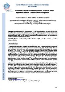
NUMERICAL TOOL FOR FLOW ANALYSIS Geometric Model The can-type atmospheric combustor (Fig. 1) developed by Morris [20] for combustion research is considered in this study. The combustor has ten curved (45) swirler passages, six primary holes, 12 secondary holes and ten dilution holes. The combustor has a length of 174.8 mm and a diameter of 82.4 mm. The fuel nozzle and spray is modelled from experimental data with a discrete drop model (see sections C and D). This research combustor will be used as a preliminary design model, and as a basis for the optimisation study. Since the configuration is symmetrical, only half of the geometry was modelled. Due to the complexity of the geometry and automation required by the optimisation method, the physical domain has been discretised using an unstructured tetrahedral mesh. It was found from a sensitivity study that 500 000 computational cells provided an adequate accuracy and speed. Since geometric modelling and grid generation are the most time-consuming and labourintensive processes in CFD-based design systems, the Gambit journalling toolkit has been intensively used to repeat model building for different CFD sessions. The procedures were written in parametric form, such that when a variation of a particular analysis case is generated, one only needs to change the value in the parameter file, and then re-run the procedures. A flow diagram of the iterative optimisation procedure is shown in Fig. 2. For every iteration or given starting design xi, i=1,2,3…, the mathematical optimiser generates a new set of variables that

6

needs to be evaluated. A journal file is then generated with the current variables and passed to the pre-processor to generate the mesh used in the solver. After the CFD simulation has converged, a file is written to a hard disk, which is then processed to derive the data that will be processed with the numerical integrating code to yield the objective function. The mathematical optimiser obtains all the data, sets up a new approximate optimisation subproblem P(i), and computes the associated new optimum design x*(i). For the next iteration i:=i+1, the new starting design is set at x(i):= x*(i-1) and the new subproblem is constructed and solved. This process is repeated until convergence to the global optimum x* is obtained. With this implementation, the time required to generate an improved geometry has been reduced from the order of days to minutes.

Boundary Conditions Boundary conditions that need to be specified are the mass flow inlets through the swirler, primary holes, secondary holes and dilution holes. The combustor outlet plane is modelled as a pressure outlet boundary. The symmetry boundary planes are modelled as rotational periodic boundary conditions. The air flow distribution boundary conditions were obtained from measurements and are shown in Table 1 [20]. The total mass flow rate of air into the combustor is 0.1 kg/s. The mass flow splits are as follows: 8.4% through the swirler, 12.5% through the primary holes, 15.3% through the secondary holes and 60.5% through the dilution holes.

Fuel Spray Droplet Dispersion Model In gas turbine combustion chambers, the fuel nozzle is of major importance for the flow and mixture field in the primary zone. CFD analysis of the fuel film dynamics and atomisation

7

process has not reached a sufficiently matured state for design purposes [21]. Due to this limitation, a more feasible approach in which fuel is injected at the pre-filmer exit with a prescribed size and velocity distribution is used. The droplets are tracked in physical space with drag and evaporation models. A Lagrangian approach is used to represent a collection of droplets having the same physical attributes such as position, velocity, temperature and diameter. The droplets and gas interact by exchanging mass, momentum and energy [22]. The actions of the gas phase on the liquid phase are introduced through the drag function terms in the liquid-phase momentum equations, and the heat transfer terms in the liquid-phase energy and mass conservation. Heat and mass transfer between droplets and gas phases are modelled by the RanzMarshall relations which describe the Nusselt and Sherwood numbers as functions of droplet Reynolds, Prandtl and Schmidt numbers. The evaporation rate is given by the Frossling correlation [23]. Details of the numerical procedure and models for the drag and evaporation can be found in references [24, 25]. In order to form a spray from the droplets, the mass flow rate of the fuel injected is divided among a prescribed number of sizes, positions and velocities given in Table 2. Each droplet pack is assigned initial conditions of size, position and velocity. The input data forms a cone with a half angle 40.

Fuel Spray Injection Model Considering that a spray consists of a huge number of drops, it is common practice to gather similar droplets (same diameter, velocity and liquid properties) in a parcel and calculate the trajectory of the parcel to represent that category of drops. This approach (known as the discrete droplet model) [26] is widely used in CFD softwares and was used in the current study. Fluent Inc [25] has implemented both the atomiser and non-atomiser models in their code for spray modelling. In the present study, due to insufficient information on the dimensions of the

8

atomiser, a spray from the atomiser had to be characterised experimentally for the discrete phase modelling. The drop breakup and atomisation processes are not modelled and the liquid spray is assumed to be thin permitting volume displacement [27], and other thick spray effects are not present [28]. If the spray cannot be considered dilute, it might affect the properties of the carrier fluid. In this case, the spray is dense enough to affect the carrier flow field via momentum exchange between the droplets and the carrier fluid. The liquid is assumed to enter the combustor as a fully atomised spray comprised of spherical droplets. In order to characterise the spray for CFD modelling, a Malvern instrument phase doppler particle analyzer (model 2600) was used to obtain the droplet size and distribution of the spray. The spray measurements were taken at a pressure of 825 kPa, which produced a flow rate of 0.77 g/s. The nozzle used was a Malvern 1.0 USGPH, 80 R. This nozzle produced a solid cone spray. A 300 mm focal length lens that made the instrument sensitive to droplets of between 5.8 and 564 m in diameter was used to take the measurements. The data was taken at room temperature and pressure, and the fluid used was kerosene. The density, surface tension, and dynamic viscosity of this fluid at standard pressure and temperature were780 kg/m3, 0.0263 N/m and 0.0024 kg/m.s. The fuel spray model uses a Rossin-Rammler [29] drop size distribution function as shown in Fig. 3, characterised by a minimum diameter of 5.8 m, a Sauter mean diameter (SMD) of 27.37 m, a maximum drop size of 204 m, drop size parameter (X) = 38 m and a drop size spread parameter of 1.78. The droplets were divided into 16 different size ranges and are introduced into the combustor at 36 discrete circumferential injection points equally spaced at the centre of the combustor. Table 2 shows the discretised fuel spray data used for the CFD spray model. The non-atomiser model used involves building a cone. A cone was constructed for 5, 12, 19, 26, 32,

9

and 40 degrees with spray boundary conditions given in Table 2. The injection velocity for all droplets was 32.5 m/s.

Consistency and Convergence It was not possible to perform strict consistency tests, because of the heavy computations that are required. However, a compromise was found between the number of cells (grid size) that gives satisfactory accuracy within a reasonable time for the design optimisation study. In a consistency test, it is expected that as the grid is shrunk indefinitely, the accuracy of the original partial differential equation is recovered. This drives the process to an unconditionally consistent numerical scheme. The convergence matrix used for the analysis is based upon flow field parameters as opposed to solver residuals. Convergence of the combusting flow field is demonstrated when the area-weighted temperature at the combustor exit plane remains unchanged for 1000 iterations.

Computational Approach Commercial software [25] was used to perform the numerical analyses of the study. The selected pre-processor, GAMBIT, acts both as a geometry modeller and mesh generator. The CFD code solves the gas equations in Eulerian form whereas the droplets are treated in a Lagrangian formulation with discrete trajectories. The spherical droplets evaporate according to the uniform temperature model [23] and interchange enthalpy, mass and momentum with the gas phase and vice versa. The main local temperature is calculated along the lines of the assumed probability density function (PDF) approach (f-g model) [30] by weighting the mixture fraction-dependent thermodynamic equilibrium temperature with an assumed probability density function. This twoparameter solely depends on the local average of the mixture fraction and its variance which was

10

assumed to be a -function. This approach applies specifically to the simulation of turbulent diffusion flames. Turbulence was modelled using the standard k- model along with wall functions for the treatment of the near-wall regions. The standard k- model has limitations in capturing regions of strong stream-wise curvatures, as well as vortices and boundary layer separation. However, the model is computationally inexpensive, which makes it ideal for this design optimisation study. This is necessitated by the fact that the work involves many CFD simulations that take long to converge. To reduce the computational effort, the following further simplifications have been implemented: the effects of buoyancy forces have been neglected so that only a periodic portion of the domain is analysed, the pressure variations are so small that the flow has been considered incompressible, and due to the fact that this is an atmospheric combustor whereby soot particles will be small in diameter, radiation has also been neglected [4]. For the mixture fraction/PDFmodel a PDF file was generated with a Pre-PDF processor. The PDF file was imported into the solver to set up the solver case file. The PDF file contains a lookup table needed by the mixture fraction/PDF model. The equilibrium mixture calculated by the PDF model was assumed to consist of nine different species and radicals: C13H24, CO2, N2, O2, H2O, CO, H2, O, and OH. Since the commercial CFD code used for this study was applicable to a wide range of engineering problems, it was necessary to customise the physical submodels and numerical methods and to streamline the boundary condition specification for the current application. To eliminate repetitive input and/or automate various tasks and to speed up parametric studies of different designs, a journal file was developed. For continuous-phase calculations, SIMPLE [25] method and an algebraic multigrid solver [25] were used. In this application, numerical accuracy

11

provided by first-order approximation is insufficient, so second-order accurate approximations were used. In numerical mathematics terms, this is performed by introducing differences that provide additional terms otherwise appearing in the truncation error. The second-order upwind scheme [25] for all scalar equation was used for discretisation.

Validation To ensure that computational fluid dynamics modelling is correct, it is necessary to validate the simulation results against accurate and reliable experimental results. This validation process assures the user that the code can be used with confidence for simulations and the user can use the code in the correct manner to solve the problem. In this validation study, simulation results were compared with experimental results of a Berl combustor model [31]. A standard k-e model was investigated to assess its accuracy on reacting flows in a combustor. The test case study was performed following “Best Practice Advice for Combustion and Heat Transfer”, [31], however, critical model configurations were made where necessary. The above reference observes the fact that stringent environmental legislation requires very low NOx and CO, a more efficient methodology to design a cleaner system is needed, and computational fluid dynamics reduces experimental costs. In this reference, there are some references to documented underlying flow regimes in a knowledgeable base, one of which is “Bluff Body Burner for CH4H2 turbulent combustion”. The validation was performed on an unstaged natural gas flame in a 300 kW industrial burner shown in Fig. 4. The experimental results of this work were collected from Sayre et al. [32]. The burner features 24 radial fuel ports and a bluff centre-body. Air is introduced through an annular inlet and movable swirl blocks are used to impart swirl.

12

The simulations code solves the equations for conservation of momentum, conservation of mass, energy and species concentrations. The reaction was modelled with a mixture fraction/PDF model and radiation was modelled with a P-1 model. The standard wall functions were used with this model. Since it was the model error that was important to determine, the calculations were performed to minimise the iterative errors and discretisation errors, i.e. make sure the solutions were converged and independent of the grid.

Case set-up A commercial computational fluid dynamics code [25] for turbulent reacting flows was used to carry out all flow analyses. The three-dimensional features (radial fuel ports) were considered in all numerical computations and a 1/24 sector of the combustor was modelled. The flow also includes strong streamline curvatures, as well as vortices and boundary layer separation. The standard k-e model was used for the validation study. The mixture fraction/PDF was used to model chemical reactions. In this approach, the transport equations for mixture fraction and its variance are solved, instead of the species equations. The density and the component concentrations are derived from the predicted mixture fraction and the variance distributions. This approach applies specifically to the simulation of turbulent diffusion flames. To reduce the computational efforts, further simplifications have been considered: the effects of the buoyancy forces have been neglected, so that only the symmetric portion of the domain was analysed; the pressure variations are so small that the flow has been considered incompressible and wall functions have been used to model the near-wall region. As a requirement of the mixture fraction/PDF model, a PDF file was set up with a pre-PDF processor. Then the PDF file was imported into the commercial CFD code to setup a case file. The PDF file contains a look-up table needed by the mixture fraction/PDF model in the CFD

13

code. The equilibrium mixture for calculation with PDF model was assumed to consist of 13 different species and radicals: CH4, C2H6, C3H8, C4H10, CO2, N2, O2, H2O, CO, H2, O, OH and H. Turbulent Prandtl and Schmidt numbers were set to 0.7 and 0.25, respectively. These values provided a better fit of predictions to experimental values. Other researchers [7, 33] have used similar values in their predictions. Sivaramakrishna et al. [33] argues that the main emphasis should be on keeping both Prandtl and Schmidt numbers unchanged, and not trying to fit the CFD simulations to experimental results by varying the values.

Velocity Profiles The comparisons of velocity profiles were made along three lines across the combustor at axial distances of 27 mm and 109 mm from the quarl body. The quantities on which comparisons are made are velocity profiles and temperature profiles for numerical predictions and measurements results. In Fig. 5 and 6, the axial velocity is plotted against the crosswise direction. The results in Fig. 5 show that the curve for the numerical predictions has good agreement with the measurements in shape. At a greater radius, the numerical predictions gave the results close to the measurements. This model underpredicted the strength of the reverse flow velocity near the centreline, however, the peak velocities are overpredicted. In Fig. 6, the numerical predictions have predicted recirculation (negative velocity) and its curve has the same shape as the measurements. It has predicted velocities close to measurements near the centreline, but, as the results move away from the centreline, the predictions deteriorate. The peak velocity has, however, been overpredicted with peaks appearing at a smaller radius.

14

Temperature Profiles Temperature calculation is very important in combustion. For a swirling flow, the calculation is more difficult. In order to calculate correct temperature distributions in reacting flows, the model used should be able to calculate “correct” velocities in non-reacting flows and this gives some problems for most of the numerical codes. Figure 7 shows the temperature contours in the combustor from which the plots of temperature at different locations were derived. Figures 8 and 9 show curves of temperature plotted against radius for the three axial locations (27 mm and 109 mm). In Fig. 8, the numerical predictions have predicted the temperature satisfactorily near the centreline, and over-predicted the peak temperatures. However, the curve has the same shape as the curve for measurements. The PDF model used shows the presence of sharp spikes, and the cause can be an inherent limitation of the numerical model [25]. The limitation results from peak temperature predictions in a narrow region where the stoichiometry is achieved according to the mixture field [25]. In Fig. 9, the numerical predictions near the centerline are acceptable, but the same spiky behaviour of the PDF model is evident. Peak temperatures have been overpredicted. However, the predicted curve fairly resembles the experimental curve. The difference between the measurements and numerical predictions on the location x-axis = 0 (in the vicinity of the wall) is minimal for all the locations (i.e. 27 mm and 109 mm) and falls within 200 K, which is a 10% difference. When looking at the temperature profiles, there are differences in both minimum and maximum temperature shown by measurements and predictions, but the profiles represent each other favourably. A similar relationship has been shown by reference [25], when using the same combustor to model flow and heat transfer. The predictions show a longer and thinner flame than as observed in measurements. The minimum

15

temperature recorded has been significantly overpredicted by 290 K at 27 mm, and this exists at the sharp spike.

Turbulence models Although only the results of the standard k-ε turbulence model were given in this study, other models were also tested. They were the renormalization-group k-ε model, realizable k-ε model, and Reynolds stress method. It has been found, however, that the standard k-ε model is of adequate accuracy, robust enough and computationally efficient in the simulation of diffusion flame.

Conclusions The agreement between the measurements and numerical results for velocity and temperature are satisfactory. The curves for numerical predictions have good agreement with the measurement in shape, but the accuracy in other locations is unsatisfactory. Inherent limitations in the CFD code resulted in-accuracies, and one of them is the assumption of equilibrium chemistry in the PDF model [33, 34, 35]. Other errors could arise from modelling turbulence with standard k-e model and choices of Prandtl and Schmidt number [33]. Lastly errors could occur due to lack of precision in boundary condition and also errors in measurements. The difference between CFD predictions and measurement for both velocity and temperature are consistent with literature [34], especially the fact that trends are very representative. Basing on the above results, it is therefore, assumed that numerical predictions can be used for modeling diffusion flames. The computational speed of the standard k-ε model makes it a good candidate for this computationally expensive study.

16

COMBUSTOR NUMERICAL FLOW FIELDS

The CFD results of the velocity vectors on the longitudinal planar section on the symmetry plane of the combustor are shown in Fig. 10. The plots display the swirling flow, primary, the secondary and dilution penetration. The primary zone is located between the swirlers and primary holes. The recirculation zone in the combustor primary zone is caused by the joint effect of the primary jet impingement and the shearing, upstream of the jet. The mixing and recirculation in this zone provide an ideal aerodynamic condition for evaporation of the fuel spray and ignition of the mixture. The near-unity equivalence ratio created in the primary zone is an important factor in promoting the flame stability and the complete combustion of the fuel-air mixture. Satisfactory combustion is achieved when the spray is enclosed in the swirling recirculation zone. Actually, the swirling recirculation is designed to induce combustion products to flow upstream to meet and merge with the incoming fuel and air. This action also assists in stabilising the flame. When sprays are trapped in recirculation zones, droplets are sufficiently mixed with the high temperature gas, heated by the surrounding area and vaporised, and finally react with the air. Otherwise, the combustion is incomplete due to the poor distribution and mixing. When the spray is within the recirculation zone, the evaporation of droplets and the combustion of mixtures are complete, resulting in a uniform exit temperature distribution. For the current study, the central toroidal recirculation zone (CTRZ) shifted slightly off-axis near the location of the primary jet injection and might not have trapped all the spray droplets. According to Durbin et al. [33], this is a sign of low swirl and it is caused by the absence of vortex breakdown due to low swirl. The presence of a corner recirculation zone (CRZ) is also a sign of low swirl and when swirl is high, the corner recirculation zone becomes negligible. The

17

corner recirculation zone is caused by the fact that the tangential velocity distribution at the swirl exit is such that the peak velocity occurs radially outwards away from the centreline. This peak in tangential velocity profile towards the corner results in a strong primary corner recirculation zone in conjunction with a weak toroidal recirculation zone. In the high-swirl case, the flow expands rapidly soon after entering the combustor, unlike the low-swirl case. This divergence of streamlines in the high-swirl case leads to the reduction in size of the corner recirculation zone as compared to low-swirl. A carefully controlled primary flow field creates an on-axis toroidal recirculation zone, unlike in the current case where the on-axis toroidal recirculation zone has not been achieved. Due to the lack of optimised flow fields, a non-uniform combustor exit temperature profile (Fig. 11) has resulted, and in order to get a uniform combustor exit temperature profile, the combustor flow fields must be carefully controlled (optimised). The pattern factor Tmax  To  / To  Ti  in Fig. 11 is 0.5, and it is the temperature traverse quality. The pattern factor can be used to assess how good the mixing at the exit of the combustor is.

MATHEMATICAL OPTIMISATION

Mathematical optimisation has been applied to numerous problems [37, 38], many of which are in the area of computational structural mechanics. CFD has not been a natural first candidate for the application of optimisation methods, due to its high CPU requirements and associated computational expense. However, CFD has become an alternative tool for assessing different combustor designs. As an optimisation tool, it has limitations in the variation of many parameters and it requires a trial-and-error simulation, of which the interpretation relies heavily on the insight of the modeller. For combustor applications, numerical optimisation can be used after the preliminary design phase and during detailed design as part of the fine-tuning process. The

18

preliminary design uses empirical and semi-empirical tools to achieve design tasks quickly [39]. After the preliminary design phase, most of the combustor requirements are fixed and critically analysed in order to perform a first comparison between achievements and targets. Empirical methods, however, exhibit limitations in a number of critical areas, particularly in scaling combustors and achieving big advances in technology levels [40]. Also, empirical methods developed for certain design concepts may not be applicable to some other novel or revolutionary combustor concepts. The lack of viable analytical models and the limited information about the underlying physical processes involved make the combustion process a suitable candidate for numerical optimisation. Mathematical optimisation tools in this regard can play a big role in screening a wide range of design variables with an automated search for the options as opposed to systematic parameter variation. In combustor designs, the application of automated optimisation is faced with multiple objectives, which are conflicting. A solution to such an application is often a compromise between the different objectives. In multi-objective optimisation, there is not even a universally accepted definition of “optimum” unlike in a single objective optimisation. The main advantage of mathematical optimisation is that the designer is unburdened from the trial-and-error process by use of an optimisation algorithm, requiring no human interaction. The designer can focus on the formulation of the design objectives and the analysis (post-processing) of the optimisation results. In addition, mathematical optimisation may lead to unexpected designs and thus to new design philosophies. Consider the constrained optimisation problem of the general mathematical form:

min f (x); x   x1, x2 ,..., xi ,..., xn  , x  Rn T

subject to constraints:

g j (x)  0; j  1, 2,..., m hk (x)  0; k  1, 2,..., p  n

(1)

(2)

19

where f(x), gj(x) and hk(x) are scalar functions of the n-dimensional vector x. The function f(x) is the objective function that is being minimised. The gj(x) denotes the inequality constraint functions and hk(x) the equality constraint functions. The components xi, i=1,2,…,n of x are called the design variables. The optimum vector x that solves the above problem is denoted by x*:

x*   x1* , x2* ,..., xn* 

T

(3)

The optimisation problem formulated in (1)-(2) may be solved using many different gradientbased methods, such as the successive approximation sequential quadratic programming (SQP) method, or stochastic methods such as genetic algorithms. Genetic algorithms are often found to be too expensive in terms of the number of function evaluations (simulations) when compared with SQP [41-42]. The method of choice for the work done here is the relatively new gradientbased and successive approximation Dynamic-Q method [16]. The Dynamic-Q method has been extensively tested by Snyman and Hay [16] and was found to offer equal competitiveness to that of SQP. Dynamic-Q was also found to be superior to SQP at handling problems with severe noise by Els and Uys [43]. Dynamic-Q was successively applied to a mixed integer problem by Visser and De Kock [44], and this is of particular interest since the problem considered in this study is also of mixed integer nature. Dynamic-Q [16] involves the application of the dynamic trajectory method (LFOP) for unconstrained optimisation, which is adapted to handle constrained problems through an appropriate penalty function formulation [45]. In Dynamic-Q, the dynamic trajectory method is applied to successive approximate spherically quadratic subproblems of the original problem constructed from appropriate sampling of the objective and constraint functions and their gradients. Here use is made of finite forward differencing to obtain gradients of the objective and

20

constraint functions, which implies that n + 1 simulations are required per design optimisation iteration. The method also employs a fixed move limit on each variable to improve the convergence. For any general optimisation problem of the form (1)-(2), the associated penalty function formulation which transforms the constrained problem to an unconstrained problem is: min Q(x) with respect to x, where

Q(x)  f (x)   j 1  j g 2j (x)  k 1 k hk2 (x) (4) m

p

 0 if g j ( x )0 where     j  j if g j ( x )0

For simplicity, the penalty parameters  j and  k usually take on the same large positive value

 j   k   . It can be shown that as  tends to infinity, the unconstrained minimum of Q(x) yields the solution to the constrained optimisation problem. The LFOP dynamic trajectory method is applied to the penalty function formulation of the constrained problem in three phases [45]. In the Dynamic-Q approach, successive subproblems P(i), i=1,2,… are generated (see Fig. 2), at successive approximations xi to the solution x*, by constructing spherically quadratic approximations f (x), g (x) and h (x) to f(x), gj(x) and hk(x). These approximations, evaluated at the point xi, are given by 1 f (x)  f (xi )  T f (xi )(x  xi )  (x  xi )T A(x  xi ) 2 1 g j (x)  g j (xi )  T g j (xi )(x  xi )  (x  xi )T B j (x  xi ) 2 1 hk (x)  hk (xi )  T hk (xi )(x  xi )  (x  xi )T Ck (x  xi ) 2

(5)

21

where j =1,…, m, and k = 1,…, p, with the Hessian matrices A, Bj and Ck taking on the simple forms A  diag (a, a,..., a)  aI , B j  b j I , Ck  ck I

(6)

Clearly, the identical curvature entries along the diagonal of the Hessian matrices indicate that the approximate subproblems P(i) are indeed spherically quadratic. For the first subproblem (i = 1), a linear approximation is formed by setting the curvatures a, bj and ck to zero. Thereafter, a, bj and ck are chosen so that the approximating functions in expressions (5) interpolate their corresponding actual functions at both xi and xi-1. These conditions imply that for i = 2,3,…, a

bj  ck 

2  f (xi 1 )  f (xi )  T f ( xi )( xi 1  xi )  xi 1  xi

2

2  g j (xi 1 )  g j (xi )  T g j (xi )(xi 1  xi )  xi 1  xi

2

(7)

2  hk (xi 1 )  hk (xi )  T hk (xi )(xi 1  xi )  xi 1  xi

2

As already stated if the gradient vectors f, gj and hk are not known analytically, they may be approximated from functional data by means of the first-order forward differencing scheme 

In many optimisation problems, additional simple side constraints of the form kˆi  xi  ki j 

occur. Constants kˆi and k i , respectively, are lower and upper bounds for variables xi. Since these constraints are of a simple form (having zero curvature), they need not be approximated in the Dynamic-Q method and are instead explicitly treated as special linear inequality constraints.

22

As a further aid in controlling convergence, intermediate move limits are imposed on the design variables during the minimisation of the subproblem. For each approximate subproblem P(i), these move limits take the form of additional inequality constraints [11]. These inequality constraints are described by x j  x (ji 1)   j  0, x (ji 1)  x j   j  0,

j=1,2,…,n

(8)

where δj are user-specified move limits. The Dynamic-Q algorithm can be stated as follows (see Fig. 2) [16]: 1. Choose a starting point x1 and move limits j, j:=1,2,…,n and set i:=1. 2. Evaluate f(xi), gj(xi) and hj(xi) as well as  f(xi), gj(xi) and hj(xi). If termination criteria are satisfied then set x*:= xi and stop. 3. Construct a local approximate subproblem P[i] with corresponding penalty function Q(x) at xi (as in (4)), using approximations and constraints given by (4) - (8). 4. Solve the approximated subproblem P[i] to give xi by using LFOPC [45]. 5. Set i: = i + 1, xi: = x(i-1) and return to Step 2. The computational time required for one CFD simulation on a Pentium IV (with 1 Gig Ram and 2.6 Hertz) was four days. For two design variables (Case 1) and five design variables (Case 2), the computational times required at each design point x to determine all the components of the objective and constraints gradient vector, were 12 and 24 days, respectively. Since optimisation is an iterative process (see Fig. 2), the total optimisation time was so high as to make automatic linking of Dynamic-Q and CFD infeasible. Therefore, CFD simulations were performed simultaneously on a few computers from which the approximations of the objective and constraint functions were obtained. The approximate subproblems (P(i)), were then solved with

23

Dynamic-Q algorithm that is implemented in the Toolkit for Design Optimisation (TDO) software [46]. This procedure reduced the required computational time by a factor of 3 for two design variables and by 6 for five design variables.

OPTIMISATION PROBLEMS Two design variables (Case 1) This case considers the widely used approach of optimising combustor exit temperature profile by selecting dilution hole parameters as design variables [4], specifically, the number of dilution holes and the diameter of dilution holes. The number of dilution holes were allowed to vary between two and seven and the diameter between four and eight. Therefore, the limits are set as 2  x1  7 and 4  x2  8, where x1 = number of dilution holes and x2 = diameter of dilution holes. The explicit optimisation problem is therefore: Minimise f(x) = Shaded Area in Fig. 11 such that: x1 an integer, x2  R The original combustor exit temperature profile in Fig. 11, was generated with initial (starting) values of

x1 = 5 and x2 = 6. The move limits for x1 and x2 are 2 and 1, respectively, and the

perturbation sizes for calculating gradients are 1 and 0.4, respectively. No explicit inequality or equality constraints have been used, so that the minimum found is essentially for an unconstrained problem, although limits have been set on design variables so as to ensure that the problem remains realistic. The integer solutions were selected by the rounding off of the continuous approximate solution obtained.

24

Five design variables (Case 2) In this case, five design variables are considered for design optimisation and the variables are: the radius of primary holes (x1), number of primary holes (x2), number of dilution holes (x3), radius of dilution holes (x4) and swirler angle (x5). The primary hole parameters and swirler angle are considered because the recirculation zone has a tremendous effect on combustion of which the combustor exit temperature profile is a result. The optimisation parameters for Case 2 are given in Table 3. An inequality constraint is imposed so that the pressure drop does not exceed the initial pressure drop by 8% (∆p ≤ 160). The formulation of the optimisation problem is now as follows: Minimise f(x) = Shaded Area in Fig. 11 such that: g1  p  160  0 (inequality constraint) g j   x j  x min  0, j

j  1, 2,...,5

g j  2   x j  x max  0, j

j  1, 2,...,5

where x min and x max denote the upper and lower limits on the variation of variables. In addition, j j move limits (Table 3) are also imposed. Here x2, x3 are integers, and x1, x4,  R The design variable x5 (swirler angle) is of different dimension and expressed in a different unit than the other four design variables. It is, therefore, necessary to scale x5 so that difficulties in calculating numerical gradients and the distortion of the objective function can be avoided. The design variable x5 is scaled through the use of range equalisation factors () as shown below:

i 

x5i  x5 LL R

,R

x5HH  x5LL

(14)

i =1,2,3,…….n.

25

where R represents the range width, HH represents the higher limit and LL represents the lower limit. Due to the scaling process, the new limits of variable x5 are; 0  x5 5.

SIMULATION AND OPTIMISATION RESULTS

The results obtained from both the CFD simulations and optimisation runs are discussed in this section. Figure 12 shows the target exit temperature profile and the original exit temperature profile for the non-optimized case. The two curves differ considerably in shape. According to Morris [20], that is because the flow splits were not optimised during the preliminary design.

Two design variables (Case 1) The results of the optimised combustor exit temperature profile are shown in Fig. 12 for Case 1, where two variables are used. In this figure, the corresponding target, optimised and nonoptimised combustor exit temperature profiles are shown. A comparison of the non-optimised and the optimised combustor exit temperature profiles shows an improvement, because the severe sinusoidal nature of the non-optimised (original) combustor exit temperature profile has been lessened. Though the optimised exit temperature profile is still not very close to the target exit temperature profile, the combustor exit temperature profile is more uniform than before optimisation. The area-weighted average of C12H23 (UHC) at the exit of the combustor was zero (0) before optimisation and zero (0) after optimisation. For CO, the area-weighted average was 0.00035 before optimisation and 0.0034 (2.8% difference) after optimisation, and this shows that CO is almost constant. The presence of CO is due to dissociation in the high-temperature combustion zone, as confirmed by the non-existence of C12H23, which can be interpreted as

26

complete combustion. The pattern factor was 0.50 before design optimisation and 0.36 after design optimisation, showing some improvement. Figure 13 shows the optimisation history of the objective function. The objective function essentially levels out after seven design iterations, showing that the objective function has converged. The objective function has apparently converged to a local optimum, with the global optimum for this case probably corresponding to the lower value (F=4.8) of the objective function reached at iteration six (see Fig. 13). The objective function has decreased from 5.3 to 4.8 at iteration six, which represents a decrease of 9.4% and corresponds to a feasible design. At this minimum value of the objective function, the design variables are given as x1 = 4 (number of dilution holes), and x2 = 4 (diameter of dilution holes) as shown in Fig. 14. It can be observed in Fig. 14 that the design variables are still changing after the eighth iteration, although the objective function in Fig. 13 has levelled off. This indicates that the last three designs in the optimisation run are effectively equivalent having the same objective function value (shaded area between the two curves), although the design variables differ slightly. Figure 15 shows the exit temperature contours on the centre plane (left side) and outlet plane (right side) of the combustor for both non-optimised (Fig. 15a) and optimised (Fig. 15b) cases. The exit temperature contours in Fig. 15b are better than in Fig. 15a. In Fig. 15a, there is a hot section in the centre and a cold section mid-way and a variation of cold and hot sections close to the wall of the combustor. This is caused by poor mixing due to the non-optimised number and diameter of dilution jets, and mixing is improved in Fig. 15b. The left sides of Fig. 15a and Fig. 15b show how the jet penetrates the combustor. It can be noticed that the jet in

Fig. 15a

underpenetrates, whereas the one in Fig. 15b penetrates deeper into the combustor causing an

27

improvement in mixing. The pattern factor for Case 1 has improved from 0.50 (Fig. 11) to 0.36 (Fig. 12) and this has the possibility of prolonging the life of turbine blades. In Case 1, the pressure drop has increased by 37% from the original value, which is an undesirable feature, though it is beneficial to combustion and dilution processes. This is because a high pressure drop results in high injection air velocities, steep penetration angles, and a high level of turbulence, which promotes good mixing [4]. These results show that the optimum design creates a higher pressure drop in the combustor, and therefore, would be difficult for the design to be improved without using other design parameters without increasing pressure drop. Due to the fact that high pressure loss was experienced in Case 1, a pressure loss constraint was imposed in Case 2.

Five design variables (Case 2) The results of the optimised combustor exit temperature profile for Case 2 with five design variables are shown in Fig. 16. In this figure, the corresponding target, optimised and nonoptimised combustor exit temperatures are shown. A comparison of the non-optimised and the optimised combustor exit temperature shows an improvement, because the optimised combustor exit temperature profile is more uniform than the original exit temperature profile. Although the combustor exit temperature profile is improved by optimisation, the pattern factor has increased from 0.50 to 0.55. The area-weighted average of C12H23 or unburnt hydrocarbons (UHC) at the exit of the combustor was zero (0) before optimisation and zero (0) after optimisation. For CO, the area-weighted average was 0.00035 before optimisation and 0.00034 (2.9% difference) after optimisation, and this shows that CO is almost constant. As in Case 1, the presence of CO is due to the dissociation in the high-temperature combustion zone, as confirmed by the non-existence of C12H23, which can be interpreted as complete combustion.

28

Figure 17 shows the optimisation history of the objective function. It can be noticed that the objective function essentially levels out after nine design iterations, showing that the objective function has converged to a local minimum. Again the objective function has probably reached the neighbourhood of the global minimum at iteration eight where it attains the value of 3.9, representing a decrease of 26% relative to its initial value of 5.3. At this minimum objective function value, the design is feasible (see Fig. 19) with variables given as x1 = 3.9 (diameter of primary holes), x2 = 2 (number of primary holes), x3 = 3 (number of dilution holes), x4 = 4.3 (diameter of dilution holes) and x5 = 47.3° (swirler angle). In Fig. 18, it can be observed that some design variables are still changing (though with small magnitudes) after the ninth iteration, although the objective function has almost levelled off. This indicates that the last three designs in the optimisation run are effectively equivalent having almost the same objective function values (shaded area between the two curves), although their geometries differ slightly. Figure 19 shows that during the optimisation, the pressure drop (inequality constraint) mostly remained within the limit imposed by the inequality constraint. The inequality constraint was violated during iteration three when it exceeded zero and for the iterations that followed, the designs remained feasible. Figure 20 shows the temperature contours of the combustor exit plane for both the non-optimised and the optimised cases. The combustor exit temperature contours in Fig. 20b are better than in Fig. 20a. In Fig 20a, there is a hot section in the centre and a cold section midway and a variation of cold and hot sections close to the wall of the combustor. This is caused by poor mixing due to an unoptimised flow field, which is improved in Fig. 20b. The purpose of optimising the swirler angle and the diameter of the primary holes was due to the fact that the primary zone flow field has some effects on the combustor exit temperature profile. Figure 21 shows the non-optimised and optimised swirl velocity. The swirl velocity for the

29

optimised case is increased, hence, modifying the size of the central toroidal recirculation zone. The central toroidal recirculation zone is also a function of the interaction of the swirling flow and the size and the number of primary holes [4, 47]. Decreasing the number of holes and increasing the diameter of the holes increase the size of the central toroidal recirculation zone [4]. In this case, the optimiser increased the swirl velocity (by increasing the swirl angle) and provided bigger and fewer primary holes. This has the effect of increasing the size of the central toroidal recirculation zone. The formation of the central toroidal recirculation zone is shown in Fig. 22. The optimised Case 2 has high peaks of positive and negative axial velocity. Very high values of swirl are, however, not appreciated because the flame can be located very close to the nozzle and dome, causing damage to them and it also affects flame stability [4]. This interaction has subsequent influences on emissions. This requires tight limits on the swirler and primary hole parameters and could also limit the inclusion of these parameters in the optimisation problem. Therefore, care must be taken when selecting the limits of the design variables related to the swirler and the primary holes, particularly when dealing with reacting flows.

CONCLUSION

This paper has shown that CFD and mathematical optimisation can successfully be combined in gas turbine combustor design optimisation. The methodology was used to obtain a more uniform combustor exit temperature profile by optimising the combustor with two dilution hole variables for Case 1 and five design variables (for dilution holes, secondary holes and swirler) for Case 2. Increasing design variables from two (Case 1) to five (Case 2) provided optimum results that fell within acceptable limits of pressure drop. The optimiser returns a significant modification in the

30

combustor exit temperature profile. The optimisation process was started with an extremely nonuniform combustor exit temperature profile, however, improved results were achieved for both cases. The methodology can be considered a supporting tool in the detailed design, complementing physical understanding as well as trial-and-error design. It should be noted that this methodology cannot replace the empirical and semi-empirical design tools for preliminary design, but it is very useful when optimising the final designs to achieve certain performance requirements. Though the method was applied to the combustor exit temperature profile, it can possibly be used for other performance requirements as long as the objective function and constraints can be written in an analytical equation or approximated function. The current results have not been validated against experimental results, but the proposed strategy was initially tested on a base case design example, on which model validation was performed with a well-researched Berl combustor before this work was carried out, in order to cultivate the ability to reproduce correct reacting flow results.

ACKNOWLEDGEMENTS The authors would like to acknowledge the contribution of Prof J. A. Visser and Mr R. M. Morris (formerly at the University of Pretoria).

31

NOMENCLATURE

aj, bj, cj

approximated curvature of objective constraint of subproblem

A, Bj, Ck

Hessian matrix

f

mixture fraction

f(x)

objective function

gj(x)

j-th inequality constraint function

hj(x)

k-th equality constraint function

I

identity matrix turbulence intensity

i

iteration

k

turbulence kinetic energy [m2/s2]

Le

turbulence length scale [m]

P(i)

approximate optimisation subproblem

p(x)

penalty function

n

R

n-dimensional real space

T

temperature [K]

x

design vector

βk

penalty parameter

ε

rate of dissipation

δj

specified move limit for i-th design variable

μi

penalty parameter

ρj

penalty parameter

kˆ

lower bound



k

upper bound

Sub-/Superscripts i

inlet

o

outlet

i,j,k

index

32

REFERENCES

[1] Qingjun, Z., Huise, W., Xiaolu, Z., and Jianzhong, X., Numerical Investigation on the Influence of Hot Streak Temperature Ratio in a High-pressure Stage of Vaneless Counter-rotating Turbine, International Journal of Rotating Machinery, Vol. 2007, 2007. [2] Barringer, M.D., Thole, K.A., and Polanka, M.D., Effects of Combustor Exit Profiles on High Pressure Turbine Vane Aerodynamics and Heat Transfer. Proc. ASME Turbo Expo Conf., Barcelona, paper GT2006-90277, 2006. [3] Mongia, H. C., A Synopsis of Gas Turbine Combustor Design Methodology Evolution of Last 25 Years, Proc. ISABE Conf., Bangalore, paper 2001-1086, 2001. [4] Lefebvre, A. H., Gas Turbine Combustion, 2nd Edition, Taylor & Fancis, Philadelphia, p. 340, 1998. [5] Lefebvre, A. H., and Norster, E. R., The Design of Tubular Gas Turbine Combustion Chambers for Optimum Mixing Performance, Proc. Institution of Mechanical Engineers, Vol. 183, pp. 150-155, 1969. [6] Holdeman, J. D., Liscinsky, D. S., Oechsle, V. L., Samuelsen, G. S., and Smith, C. E., Mixing of Multiple Jets with a Confined Subsonic Cross Flow: Part 1- Cylindrical Duct, Journal of Engineering for Gas Turbine and Power, Vol. 119, pp. 852-862, 1997. [7] Gulati, T., Tolpadi, A., and Vanduesen, G., Effect of Dillution Air on Scalar Flow Field at the Combustor Exit, Proc. ASME IGTI Conf., Arizona, paper 94-0221, 1994. [8] Tangarila, V., Tolpadi, A., Danis, A., and Mongia, H., Parametric Modeling Approach to Gas Turbine Combustor Design, Proc. ASME IGTI Conf., Munich, paper 2000-GT-0129, 2000.

33

[9] Catalano, L. A., Dadone, A., Manodoro, D., and Saporano, A., Efficient Design Optimization of Duct-burner for Combined-cycle and Cogeneration Plants, Engineering Optimisation, Vol. 38, No. 7, pp. 801-820, 2006. [10] Becz, S., and Cohen, J. M., Characterization Of Mixing For A Jet In Cross-flow Using Proper Orthogonal Decomposition, Proc. ASME TURBO EXPO Conf., Reno-Tahoe, 2005-0307, 2005. [11] Morris, R. M., Snyman, J. A., and Meyer, J. P., Jets in Crossflow Mixing Analysis Using Computational Fluid Dynamics and Mathematical Optimization, Journal of Propulsion and Power, Vol. 23, No. 3, pp. 618-628, 2007. [12] Dispierre A., Stuttaford P. J., and Rubini, P. A., Preliminary Gas Turbine Combustor Design Using a Genetic Algorithm, Proc. ASME IGTI Conf., Amsterdam, paper 97-GT72, 1997. [13] Rogero, J. M., A Genetic Algorithm Based Optimisation Tool For the Preliminary Design of Gas Turbine Combustors, Ph.D Thesis, School of Mechanical Engineering, Cranfield University, UK, 2002. [14] Zomorodian, R., Khaledi, H., and Ghofrani, M., A New Approach to Optimisation of Cogeneration Systems Using Genetic Algorithm, Proc. ASME TURBO EXPO Conf., Barcelona, paper GT2006-90952, 2006. [15] Stuttaford, P. J., and Rubini, P. A., Preliminary Gas Turbine Combustor Design Using Network Approach, Proc. ASME IGTI Conf., Birmingham, paper 96-GT-135, 1996. [16] Snyman, J. A., and Hay, A. M., The Dynamic-Q Optimization Method: An Alternative to SQP?, International Journal of Computers and Mathematics with Applications, Vol. 44, No. 12, pp. 1589-1598, 2002.

34

[17] Kingsley, T., Design Optimization of Containers for Sloshing and Impact, MSc. dissertation, University of Pretoria, Pretoria, South Africa, 2005. [18] Craig, K. J., De Kock, D. J., and Snyman J.A., Using CFD and Mathematical Optimization to Investigate Air Pollution Due to Stacks, International Journal of Numerical Mathematics in Engineering, Vol. 44, pp. 551-565, 1999. [19] De Kock, D. J., Craig, K. J., and Pretorius, C.A., Mathematical Maximisation of Minimum Residence Time for Two Strand Continuous Caster, Iron Marking and Steel Marking, Vol. 30, No. 3, pp. 229-234, 2003. [20] Morris, R. M., An Experimental and Numerical Investigation of Gas Turbine Research Combustor, MSc. dissertation, University of Pretoria, Pretoria, South Africa, 2000. [21] Custer, J. R., and Rink, N. K., Influence of Design Concept and Liquid Properties of Fuel Injection Performance, Journal of Propulsion, Vol. 4, No. 4, 1987. [22] Crowe, C. T., Sharma, M. P., and Stock, D. E., The Particle Source-In-Cell (PSI-CELL) Model for Gas-Droplet Flows, Journal of Fluids Engineering, Vol. 99, pp. 325-332, 1997. [23] Faith, G. M., Evaporation and Combustion of Sprays, Progress in Energy and Combustion Science, Vol. 9, pp. 1-76, 1983. [24] Sabnis, J.S., Gibeling, H.J., and McDonald, H.A., Combined Eulerian-Lagrangian Analysis for Computation of Two-Phase Flow, AIAA paper, 87-1419, 1987. [25] FLUENT, Software package, Ver. 6.2.16, Fluent Inc., Lebanon, NH, 2004. [26] Tap, F. A., Dean, A. J., and Van Buijttenen, J. P., Experimental and Numerical Spray Characterization of a Gas Turbine Fuel Atomizer in Cross Flow, Proc. ASME TURBO EXPO Conf., Amsterdam, paper GT-2002-30100, 2002.

35

[27] Dukowicz, J. K. A., Particle Fluid Numerical Model for Liquid Sprays,” Journal of Computational Physics, Vol. 35, pp. 229-253, 1980. [28] O’Rouke, P. J., Collective Drop Effects in Vaporizing Liquid Sprays, Ph.D thesis, Princeton University, and Los Alamos National Laboratory Report, LA-9069-T, US, 1981. [29] Rosin, P., and Rammler, R., The Laws Governing the Fineness of Powdered Coal, Inst. of Fuel, pp. 29-36, 1933. [30] Libby, P. A., and Williams, F. A., Turbulent Reacting Flow, Academic Press, 1994. [31] Fluent News, The Berl Combustor Revisited, Vp1 xii, ISSUE 1, 2003. [32] Sayre, A., Lallemant, N., Dugue, J., and Weber, R., Scaling Characteristics of Aerodynamics and Low-Nox Properties of Industrial natural Gas Burners, The Scaling 400 Study, Part IV: The 300 kW Berl Test Results, IFRF Doc No F40/y/11, International Flame Research Foundation, The Netherlands, 1996. [33] Sivaramakrishna, G., Muthuveerappan, N., Shankar, V., and Sampathkumaran, T.K., CFD Modeling of the Aero Gas Turbine Combustor. ASME Turbo Expo, 2001-GT-0063, 2001. [34] Smiljanovski, V., and Brehm, N., CFD Liquid Spray Combustion Analysis of a Single Annular Gas Turbine Combustor, Proc. ASME IGTI Conf., Indianapolis, paper, 99-GT300, 1999. [35] Fuligno, L., Micheli, D., and Poloni, Carlo., An Integrated Design Approach for Micro Gas Turbine Combustors: Preliminary 0-D and Simplified CFD Based Optimization, ASME Turbo Expo, GT2006-90542, 2006.

36

[36] Durbin, M. D., Vangsness, M. D., Balla, D. R., and Katta, V. R., Study of Flame Stability in a Step Swirl Combustor, Conf. ASME IGTI Conf., Hawaii, paper 95-GT-111, 1995. [37] Schmit, L. A., and Farshi, B., Some Approximation Concepts for structural Synthesis,” AIAA Journal, Vol. 12, No. 5, pp. 692-699, 1974. [38] Haftka, R.T., and Gurdal, Z., Elements of Structural Optimization, Kluwer Academic Publishers, Boston, p. 221, 1992. [39] Mongia, H. C., Aero-thermal Design and Analysis of gas Turbine Combustion Systems: Current Status and Future direction, Conf. ASME IGTI Conf., Cleveland, paper 98-3982, 1998. [40] Rinz, A., and Mongia, H. C., Gas Turbine Combustor Design Methodology, Conf. ASME IGTI Conf., Dusseldorf, paper 86-131, 1986. [41] Baumal, A. E., McPhee, J., and Calamai, P. H., Application of Genetic Algorithms of an Active Vehicle Suspension Design, Computer Methods in Applied Mechanics and Engineering, Vol. 163, pp. 87-94, 1998. [42] Eberhard, P., Schiehlen, W., and Bestle, D., Some Advantages of Stochastic Methods in Multi-criteria Optimization of Multibody Systems, Archive of Applied Mechanics, Vol. 69, pp. 543-554, 1998. [43] Els, P. S., and Uys, P. E., Investigation of the Applicability of the Dynamic-Q Optimisation Algorithm to Vehicle Suspension Design, Mathematical and Computer Modelling, Vol. 37, Nos. 9-10, pp. 1029-1046, 2003.

37

[44] Visser, J. A., and De Kock, D. J., Optimization of Heat Sink Mass Using the DynamicQ Numerical Optimization Method, Communications in Numerical Methods in Engineering, Vol. 18, No. 10, pp. 721-727, 2002. [45] Snyman, J. A., The LFOPC Leap-Frog Algorithm for Constrained Optimization, Computers and Mathematics with Applications, Vol. 40, pp. 1085-1096, 2000. [46] Toolkit for Design Optimization (TDO) software, version 1.2d, Department of Mechanical and Aeronautical Engineering, University of Pretoria. [47] Vanoverberche, K. P., Van Den Bulck, E. V., and Tummers, M. J., Confined Annular Swirling Jet Combustion, Combustion Science and Technology, Vol. 175, pp. 545-578, 2003.

38

Oboetswe Motsamai is a Ph.D student at the University of Pretoria, Department of Mechanical and Aeronautical Engineering, South Africa. He received the B.Eng Mechanical from the University of Botswana in 1996 and MSc Thermal Power and Fluids Engineering from the University of Manchester Institute of Science and Technology in 2000. He has previously worked for Kentz Botswana (1997) as a Junior Engineer and later worked for G4 Consulting Engineers (1998) as an Engineer. He is currently working for the University of Botswana as lecturer in the department of mechanical engineering. He is doing his research on developing a design optimization methodology for gas turbine combustors.

Jan Snyman received BSc (Hons) degrees in both physics and mathematics from the Universities of Cape Town and Pretoria respectively in 1961 and 1964, a MSc degree in physics from the University of South Africa in 1964, and the PhD degree in theoretical physics from the University of Pretoria in 1975. He started his career as a research officer at the National Physical Research Laboratory of the South African Council for Scientific and Industrial Research in Pretoria in 1962. He worked in the computer industry from 1966 to 1968, first as a programmer and then as a systems analyst at English Electric Computers and IBM respectively. In 1969 he was appointed lecturer in physics at the Pretoria Technikon and in 1971 he joined the faculty of the University of Pretoria as lecturer in the Department of Applied Mathematics where he was promoted to full professor in 1983. In 1990 he joined the Department of Mechanical Engineering where he teaches Dynamics, Numerical Methods and Mathematical Optimization at both undergraduate and graduate level. After his retirement in 2005 he has, as emeritus professor, continued to be involved in the activities of the

39

Department. Prof Snyman’s research focuses mainly on two inter-related aspects of mathematical optimization: the development of new optimization algorithms and optimization methodologies of particular importance for the solving of physical and engineering design problems, and the application thereof in design problems of practical importance to industry. He has received several prizes and awards for his research, including the Centenary Research Medal (1908-2008) of the University of Pretoria. In 2004 an honorary professorship (professor honoris causae Facultatis Mechanicae) was conferred on him by the University of Miskolc in Hungary. Prof Snyman is the author or co-author of 86 scientific journal articles and one book.

Josua Meyer obtained his B.Eng. (cum laude) in 1984, M.Eng. (cum laude) in 1986, and his Ph.D. in 1988, all in Mechanical Engineering from the University of Pretoria and is registered as a professional engineer. After his military service (1988 – 1989), he accepted a position as Associate Professor in the Department of Mechanical Engineering at the Potchefstroom University in 1990. He was Acting Head and Professor in Mechanical Engineering before accepting a position as professor in the Department of Mechanical and Manufacturing Engineering at the Rand Afrikaans University in 1994. He was Chairman of Mechanical Engineering from 1999 until the end of June 2002, after which he was appointed Professor and Head of the Department of Mechanical and Aeronautical Engineering at the University of Pretoria from 1 July 2002. At present he is the Chair of the School of Engineering. He specializes in heat transfer, fluid mechanics and

40

thermodynamic aspects of heating, ventilation and air-conditioning. He is the author and co-author of more than 250 articles, conference papers and patents and has received various prestigious awards for his research. He is also a fellow or member of various professional institutes and societies (i.e. South African Institute for Mechanical Engineers, South African Institute for Refrigeration and Air-Conditioning, American Society for Mechanical Engineers, American Society for AirConditioning, Refrigeration and Air-Conditioning) and is regularly invited to be a keynote speaker at local and international conferences. He has also received various teaching and exceptional achiever awards. He is an associate editor of Heat Transfer Engineering.

41

Table 1. Boundary conditions for the combustor inlets Inlet

Swirler Primary Secondary Dilution

Velocity Components (m/s) Radial Tangential Axial 0 0.5 0.5 -0.865 0 -0.502 -0.837 0 -0.547 -0.913 0 -0.406

I [%]

Le [10-4 m]

T [K]

10 10 10 10

1.25 1.97 1.53 3.39

300 300 300 300

42

Table 2. Discretised fuel spray data Size Mean droplet size group in group [m] 1 2 3 4 5 6 7 8 9 10 11 12 13 14 15 16

7.21 8.34 10.4 12.9 16 19.9 24.8 30.8 38.4 47.7 59.3 73.8 91.7 114 142 176

Volume fraction

Mass flow [kg/s]

0.014 0.003 0.003 0.007 0.024 0.077 0.149 0.187 0.179 0.158 0.107 0.053 0.021 0.01 0.004 0.002

1.078E-05 0.231E-05 0.231E-05 0.539E-05 1.848E-05 5.929E-05 11.473E-05 14.399E-05 13.783E-05 12.166E-05 8.239E-05 4.081E-05 1.617E-05 0.77E-05 3.08E-06 1.54E-06

43

Table 3. Optimisation parameters for Case 2 Initial values Move limits Perturbation sizes Lower limit Upper limit

x1 3.3 0.4 0.2 2.3 2.9

x2 3 2 1 2 6

x3 5 2 1 2 7

x4 6 1 0.4 4 8

x5 45 0.5 1 45 65

44

List of Figure Captions Fig. 1 Three dimensional model of the combustor Fig. 2 Flow diagram of FLUENT coupled to optimizer Fig. 3 The modified Rossin-Rammler [28] drop size distribution function of the fuel spray

Fig. 4 Two-dimensional view of burner Fig. 5 Axial velocity at 27 mm from the quarl exit Fig. 6 Axial velocity at 109 mm from the quarl exit Fig. 7 Flow field showing temperature contours Fig. 8 Temperature at 27 mm from the quarl exit Fig. 9 Temperature at 109 mm from the quarl exit Fig. 10 Flow field on the symmetry plane of the combustor Fig. 11 Non-optimised combustor exit temperature profile Fig. 12 Optimised combustor exit temperature profile for Case1, which is two design variables (number of dilution holes and diameter of dilution holes) Fig.13 Optimisation history of the objective function for Case 1 Fig. 14 Optimisation history of design variables for Case 1 Fig. 15 Temperature contours on the centre plane (left side) and exit (right side) of the combustor (a) for the non-optimised and (b) the optimised Case 1 Fig.16 Optimised combustor exit temperature profile for Case 2 Fig. 17 Optimisation history of the objective function for Case 2 Fig. 18 Optimisation history of design variables for Case 2 Fig. 19 Optimisation history of inequality constraint (pressure drop) for Case 2 Fig. 20 Temperature contours of the combustor exit plane for (a) the non-optimised and (b) the optimised for Case 2, with five design variables

45

Fig. 21 Swirl velocity at 30 mm from the dome face for the non-optimised case and the optimised Case 2 Fig. 22 Axial velocity at 30 mm from the dome face for the non-optimised case and the optimised Case 2

46

Dilution hole

Rake

Primary hole

Outlet plane

Secondary hole Swirl er 1 Three dimensional model of the combustor Fig.

47

Starting design x1, i:=1

Next iteration i:=i+1 = x*(i-1)

Optimum x*:= x*(i) Yes

Pre-processing  GAMBIT journal file

No Converged CFD Simulations

Optimisation  Set-up and solve approximate optimisation subproblem P(i) to give x*(i)

Numerical integration  Evaluate objective and constraint functions

Post-processing  Process and extract data

Fig. 2 Flow diagram of FLUENT coupled to optimiser

48

ln(x)/ln(X)

10

1

0.1 0.001

0.01

0.1

1

10

ln(1-Q)^-1

Fig. 3 The modified Rossin-Rammler [28] drop size distribution function of the fuel spray

49

Fig. 4 Two-dimensional view of burner

50

50 Axial Velocity (m/s)

40

Numerical Measurements [32]

30 20 10 0 -10 0 -20

0.1

0.2

0.3

0.4

0.5

0.6

Radial Position (m)

-30

Fig. 5 Axial velocity at 27 mm from the quarl exit

51

Axial Velocity (m/s)

40 35 30 25 20 15 10 5 0 -5 0 -10

Numerical Measurements [32]

0.1

0.2

0.3

0.4

0.5

0.6

Radial Position (m)

Fig. 6 Axial velocity at 109 mm from the quarl exit

52

Fig. 7 Flow field showing temperature contours

53

Static Temperature (K)

2500

Numerical Measurements [32]

2000 1500 1000 500 0 0

0.1

0.2

0.3

0.4

0.5

0.6

Radial Position (m)

Fig. 8 Temperature at 27 mm from the quarl exit

54

Static Temperature (K)

2500 Numerical Measurements [32]

2000 1500 1000 500 0 0

0.1

0.2 0.3 0.4 Radial Position (m)

0.5

0.6

Fig. 9 Temperature at 109 mm from the quarl exit

55

CRZ

Primary hole injections

CTRZ Secondary hole injections

Dilution hole injections

Fig. 10 Flow field on the symmetry plane of the combustor

56

Original temperature profile Target temperature profile

900

Temperature [K]

800 700 600 500 400 300 200

0

10

20 30 Radial Position [mm]

40

50

Fig. 11 Non-optimised combustor exit temperature profile

57

Target exit temperature profile Optimised exit temperature profile Non-optimised exit temperature profile

900

Temperature [K]

800 700 600 500 400 300 0

10

20

30

40

50

Radial position [mm]

Fig. 12 Optimised combustor exit temperature profile for Case1, which is two design variables (number of dilution holes and diameter of dilution holes)

58

F(x)

7 6 5 4 3 2 1 0

Lower value, F = 4.8

0

1

2

3

4 5 6 Design Iteration

7

8

9

Fig.13 Optimisation history of the objective function for Case 1

59

x1 and x2

x1: Number of dilution holes x2: Diameter of dilution holes 7 6 5 4 3 2 1 0 1

2

3

4

5

6

7

8

9

10

11

Design iteration Fig. 14 Optimisation history of design variables for Case 1

60

Colour Map

Non-optimised case

(a) Optimised Case1

(b)

Fig. 15 Temperature contours on the centre plane (left side) and exit (right side) of the combustor (a) for the non-optimised and (b) the optimised Case 1

61

Optimised exit temperature profile Target exit temperature profile Non-optimised temperature profile Temperature [K]

900 800 700 600 500 400 300 0

10

20 30 Radial position [mm]

40

50

Fig.16 Optimised combustor exit temperature profile for Case 2

62

7

F(x)

6 5 4

Lower value, F=3.9 3 0

2

4

6

8

10

12

Design iteration

Fig. 17 Optimisation history of the objective function for Case 2

63

x1,x2,x3,x4 and x5

x1: Diameter of primary holes x2: Number of primary holes x3: Number of dilution holes x4: Diameter of dilution holes x5: Swirler angle 8 7 6 5 4 3 2 1 0 -1 0 -2

2

4

6

8

10

12

Design iteration

Fig. 18 Optimisation history of design variables for Case 2

64

Inequality constarint (g(x))

10 0 -10 0 -20

2

4

6

8

10

12

feasible

-30 -40 -50 Design iteration

Fig. 19 Optimisation history of inequality constraint (pressure drop) for Case 2

.

65

Non-optimised

Optimised Case 2

case

(a)

(b)

Fig. 20 Temperature contours of the combustor exit plane for (a) the non-optimised and (b) the optimised for Case 2, with five design variables

66

Optimised Non-optimised

7

Swirl velocity (m/s)

6 5 4 3 2 1 0 -40

-30

-20

-10

0

10

20

30

40

Radial position (mm)

Fig. 21 Swirl velocity at 30 mm from the dome face for the non-optimised case and the optimised Case 2

67

Non-optimised Optimised

Axial velocity (m/s)

25 15 5 -40

-30

-20

-10 -5 0

10

20

30

40

-15 -25 Radial position (mm)

Fig. 22 Axial velocity at 30 mm from the dome face for the non-optimised case and the optimised Case 2

68