Proceedings of the International MultiConference of Engineers and Computer Scientists 2011 Vol I, IMECS 2011, March 16 - 18, 2011, Hong Kong
Optimisation of Precedence-constrained Production Sequencing and Scheduling Using Genetic Algorithms Son Duy DAO & Romeo MARIAN Abstract—This paper present the development of a Genetic Algorithm (GA) for optimisation of precedence-constrained production sequencing and scheduling problems. This class of problems requires a double optimisation - for sequencing and scheduling - at the same time. Due to nature of constraints, novel strategies for encoding chromosomes, crossover, mutation operations and handling constraints have been developed. The GA developed to solve this class of problems uses variable length chromosomes and its capability is demonstrated using a complex and realistic case study. The result obtained for the case study shows that the proposed GA is applicable to real-life precedence-constrained production sequencing and scheduling optimisation problems, which are ubiquitous to production and manufacturing environments. Index Terms—genetic algorithm, precedence-constrained sequencing and scheduling, optimisation, cutting operation
T
I. INTRODUCTION
HE precedence-constrained problems are a class of common problem facing manufacturing companies. They apply to project management, logistics, routing, assembly flow, scheduling, and networking [19]. Optimisation of precedence-constrained production sequencing and scheduling problem concerns development of the production planning by selecting what products to produce and in what order to satisfy simultaneously all of the given constraints while maximising company profit. This problem is generally described as follows: For each period of time, one company can produce a variety of products, say A1, A2, ..., An and each product has a cost to produce, a price to sell, labour requirement, material requirement and deadline. In addition, the labour, material and working capital available for production are limited. Moreover, the company has to face a number of the following constraints: any product changeover takes B hours; cost of running the company is $C/hour and has to be paid from the working capital; any product made after its deadline incurs a penalty of D% of the initial price per day; for certain period of time, at least E different products have to be produced; the company can work on one product at a time. The objective is to select what products to produce and in Manuscript received December 2010; revised January, 2011. Son Duy DAO is a postgraduate student at School of Advanced Manufacturing & Mechanical Engineering, University of South Australia, Australia (corresponding author, e-mail:
[email protected]). Romeo MARIAN, PhD is Senior Lecturer and Program Director at School of Advanced Manufacturing & Mechanical Engineering, University of South Australia, Australia (e-mail:
[email protected]).
ISBN: 978-988-18210-3-4 ISSN: 2078-0958 (Print); ISSN: 2078-0966 (Online)
what order to maximise the total profit of the company while satisfying simultaneously all above constraints. This class of problems can be considered as a multidimensional, precedence constrained, knapsack problem. The knapsack problem is a classical NP-hard problem and it has been thoroughly studied in the last few decades [21]. Although a number of production planning approaches have been developed so far, highly complex production planning or real-life planning problems have not been thoroughly solved yet and their optimal solutions are still so far from perfect due to multiplicity of constraints involved. Such constraints make the optimisation very difficult when using traditional optimisation methods and approaches. Recently, a number of researchers have applied GA to solve optimisation problems of similar complexity. However, little attention has been given to dealing with problems with solutions of variable size – accordingly, the length of chromosome encoding the solution varies. This study uses GA with novel encoding, crossover and mutation strategies to optimise the precedence-constrained production sequencing and scheduling, which permits the search for an optimum, while considering simultaneously a large number of constraints of contradictory nature which causes the solution to have variable size. The proposed strategy is illustrated by a realistic case involving complex constraints. II. LITERATURE REVIEW Sequencing and scheduling is about optimally allocating scarce resources to activities over time [6]. In 1990, Chen attempted to use an AND/OR precedence-constrained sequencing problem (PCSP) to solve assembly scheduling problem in which the precedence relations result from geometric and physical constraints of the assembled items. Similarly, Marian [12] used GA to optimise precedenceconstrained assembly sequences. In order to deal with printed circuit board assembly problem, Duman & Or [5] developed an approach which initially ignores precedence relations and solves the problem as a pure travelling salesman problem (TSP), and then it is applied to eliminate component damage in the resulting TSP tour. Recently, PCSPs in disassembly scheduling problem by modification of the two-commodity network flow model was formulated by Lambert [11]. To solve scheduling model with sequence-dependent changeover cost and precedence constraints, heuristic algorithm has been developed by He & Kusiak [8]. To solve PCSP based on supply chain planning model, Moon et al. [15] proposed GA with a priority-based encoding method. A unique reasoning approach to solve PCSPs which is based IMECS 2011
Proceedings of the International MultiConference of Engineers and Computer Scientists 2011 Vol I, IMECS 2011, March 16 - 18, 2011, Hong Kong
on artificial intelligent technique of case-based reasoning with evolutionary algorithm was developed by Su [18]. Recently, in the research of Yun & Moon [20], GA approach based on a topological sort-based representation procedure was proposed to solve precedence-constrained sequencing problems. It aims at locating the optimal sequence with the shortest travelling time among all feasible sequences. Clearly, this problem can be formulated as a traveling salesman problem with precedence constraints. For single-machine sequencing with precedence constraints, Morton & Dharan [16] developed a heuristic – algoristics - to find optimal solutions. Chekuri & Motwani [3] developed an efficient combinational 2-approximation algorithm for precedence constrained scheduling to minimize the sum of weighted completion times on a single machine. For the same problems as presented in Chekuri & Motwani [3], Azar et al. [2] considered it as a special case of the vertex cover problem and then solved it by means of vertex cover theory. To deal with problem of scheduling a set of precedence constraint tasks onto a finite number of identical processors with and without communication overhead, Yen et al. [19] proposed priority-list scheduling method to minimize the makespan. In addition, Jonsson & Shin [10] proposed a parametrized branch-and-bound algorithm for scheduling precedence-constrained tasks on a multiprocessor system to minimize the maximum task lateness in the system. Selvakumar & Siva [17] developed heuristic algorithms to obtain near optimal schedules in a reasonable amount of computation time for scheduling precedence constrained task graphs with non-negligible intertask communication onto multiprocessors. For scheduling precedence-constrained computations on message-passing systems, Al-Mouhamed & Al-Maasarani [1] proposed a class of global priority-based scheduling heuristics, called generalized list scheduling. Hary & Ozguner [8] used point-to-point networks to solve precedence-constrained task allocation for pipelined execution. However, it can be also seen from the above that research attempting to optimise both sequencing and scheduling at the same time for precedence-constrained optimisation problems, especially for the large-size or real-life problems is largely missing. In this paper, a complex and realistic mathematical model for optimisation of precedence-constrained production sequencing and scheduling is built and a GA is developed for its optimisation. A special strategy for GA implementation is developed to deal with the variability of chromosome size and feasibility of chromosome. The approach is general and applicable to real-life planning problems. III. RESEARCH METHODOLOGY The tool used to solve/optimise the precedenceconstrained production sequencing and scheduling problem is GA. Obviously, there are two elements to be optimised simultaneously: which products to produce and in what order. The major steps of the GA are presented as follows: Step 1: Chromosome encoding The feasible solutions for the problem are encoded as chromosomes. In general, each chromosome is a string containing the products to be produced and their producing
ISBN: 978-988-18210-3-4 ISSN: 2078-0958 (Print); ISSN: 2078-0966 (Online)
sequences. At first, chromosome is randomly generated as a long string of number from 1 to n, which denote the product 1 to product n, respectively. Based on the constraints in labour, material, working capital and number of products required, the length of the chromosome is cut to remove some infeasible products allocated at the end of the string. After cutting operation, the chromosome is feasible and can be used to evaluate quality of the solution further. Because of cutting operation, the length of chromosome might vary to satisfy the constraints. Step 2: Fitness function Fitness function is the total profit of the company. The fitness function is calculated for each chromosome. Step 3: Genetic operators A number of genetic operators will be developed such as crossover, mutation, evaluation, selection. It is noted that after each crossover and mutation operations, the feasibility of off-springs must be checked and then repaired if necessary. Step 4: Handling constraints Due to number of constraints involved, a chromosome has to be tested for feasibility after generation and application of genetic operators such as crossover and mutation. Step 5: Optimisation implementation The classical structure of GA is chosen to search the optimal solution in terms of total profit. Specific and challenging for this class of problems is the handling of precedence constraints. Marian et al [13], [14] developed a framework capable to encode hard precedence relations (constraints that, violated, render the solution illegal or infeasible) as constraints. However, for this class of problems a soft approach is used, in line with the character of the problem – i.e. a precedence relation, if violated (part not ready for delivery at deadline) will incur a penalty rather than rendering the sequence and schedule infeasible. A penalty implies the respective chromosome is less likely to pass in the next generation, but still may have very valuable characteristics to pass on through the evolution process. The proposed approach is explained in detail with the aid of the case study. IV. A CASE STUDY A case study is presented here to illustrate and exemplify the concepts presented in the paper, described as follows: There is a manufacturing company producing high quality customised products from specialised castings. The company can produce a variety of products, A1, A2, ..., A40. Each product has a cost to produce, a price to sell, labour requirement, material requirement and deadlines, as listed in the Table 1. Each month, the company has 650 h for production, 1100 kg of material and a working capital of $400K. Additionally: any product changeover takes 2 h; the cost of running the company is $170/h and has to be paid from the working capital; a product made after the deadline incurs a penalty of 5% of the initial price per day of delay; the company works on one product at a time; the proceedings from selling products will only be available for next month, so they should be ignored for the current planning horizon (current month); IMECS 2011
Proceedings of the International MultiConference of Engineers and Computer Scientists 2011 Vol I, IMECS 2011, March 16 - 18, 2011, Hong Kong
TABLE 1 PRODUCT INFORMATION
the company can select any mix of products to produce each month, as long as its selection contains at least 12 different ones. It is required to do the planning for next month by selecting what products to produce and in what order to maximise the profit of the company while satisfying simultaneously all constraints above. A. Modelling of the problem Considering: A manufacturing company can produce 40 different products, with details in Table 1 The labour, material and working capital available in next month are known. Determine: Which products to be produced; What is the order to produce the selected products. So that the profit of the company is maximized while all constraints are simultaneously satisfied. Conditions: Known: The labour required for product changeover, the cost of running the company, the penalty for delays; The cost of running the company has to be paid from the working capital; The proceedings from selling products will only be available for next month, so they should be ignored for the current planning horizon (current month); The company can produce any mix of products; The company must produce at least 12 different products each month. B. Genetic Algorithm Optimisation Criteria The optimisation criterion for this problem is the overall profit of the company, converted into the fitness function. The quality of the solution is assessed through its fitness value, computed for every single chromosome in every generation. Chromosome Definition Let numbers from 1 to 40 denote the corresponding products A1 to A40 to be produced. Each chromosome is generated by two stages. The first stage is to randomly generate the general chromosome, so called initial chromosome, which looks like as shown in Table 2 in which: Cells C3 - AP3 represent the sequence of the products to be produced. Cells C4 - AP4 represent the products to be produced. E.g., the value of 20 of the Cell H4 indicates that the product A20 will be produced the sixth, as shown in Cell H3. The second stage is to cut the initial chromosome based on four constraints: labor, working capital, material, minimum number of products required. The procedure is explained in the Table 3. In this Table, Cells C3-AP3 represent the sequence of the products to be produced before cutting operation; Cells C4 – AP4 - the products to be made before chromosome cutting operation; Cells C5 – AP5 - the changeover time between two different products - e.g., zero in Cell D5 indicates no changeover time (product 24 made consecutively - C4 and D4). Cell K5 indicates changeover is required when producing products 8 and then 36 (Cells J4 and K4); ISBN: 978-988-18210-3-4 ISSN: 2078-0958 (Print); ISSN: 2078-0966 (Online)
Product
Cost (K$)
Price (K$)
Labour (h)
A1 A2 A3 A4 A5 A6 A7 A8 A9 A10 A11 A12 A13 A14 A15 A16 A17 A18 A19 A20 A21 A22 A23 A24 A25 A26 A27 A28 A29 A30 A31 A32 A33 A34 A35 A36 A37 A38 A39 A40
15 21 22 8 10 13 11 3 24 23 3 6 3 10 3 14 3 2 2 1 18 16 5 19 1 4 8 12 6 6 22 1 6 16 15 23 11 17 16 11
575 127 392 172 543 97 451 122 413 260 277 477 557 191 229 432 529 159 607 265 228 103 198 64 294 343 502 578 616 196 201 449 565 60 393 304 354 108 48 265
22 25 31 31 28 36 14 25 19 23 27 13 18 35 33 19 33 30 24 24 34 32 24 15 30 30 14 28 36 31 15 25 31 15 23 25 31 17 22 21
Deadline (day of month) 30 25 10 20 25 15 30 10 25 10 25 20 5 10 25 15 5 25 10 15 25 30 25 30 15 25 20 25 30 10 15 30 5 20 10 15 20 5 30 25
Material (kg) 6 86 55 88 63 11 6 6 77 47 73 72 19 42 22 73 56 65 59 22 42 32 56 19 29 42 34 84 18 31 83 35 89 47 65 16 31 48 68 59
Cells C6 – AP6 represent the labor required to make the corresponding products. E.g., the value of Cell G6 indicates it takes 28 hours to make A16 as shown in Cell G4 (from Table 1); Cells C7 – AP7 represent the material required to produce the corresponding products. E.g. the value of Cell C7 indicates the need for 6 kg of material to produce product A24 (in Cell C4); Cells C8 – AP8 represent the cost to produce the corresponding products. E.g. the value of Cell C8 indicates it costs $15K to produce A24 (Cell C4); Cells C9 – AP9; C10 – AP10; C11 – AP11 represent the labor, material and cost consumed for corresponding products in Cells C4 – AP4. E.g. Cell C9 indicates that producing A24 consumes 15 labour hours; Cell AS3 denotes the minimum number of products required to be produced; Cell AS5 - the product changeover time in hours; Cell AS8 - the cost per hour of running company; Cell AS9 - the labor available for the next month; Cell AS10 - the material available for the next month; Cell AS11 - the working capital available; Cell AQ9 - the total labor required to produce products and production sequence shown in Cells C4 – AC4 and C3 – AC3, respectively. E.g. the total labor used is 645 hours - Cell AQ9. The value of this Cell must satisfy the labor constraint (less than or equal to 650); Cell AQ10 denotes the total amount of material required to produce the sequence shown in C4 –AA4. E.g. the amount of material used is 1095 kg (Cell AQ10). This value must satisfy the material constraint (less than or equal to 1100); Cell AQ11 - total cost of producing sequence in Cells C4-X4. The total working capital - $386.65K, Cell IMECS 2011
Proceedings of the International MultiConference of Engineers and Computer Scientists 2011 Vol I, IMECS 2011, March 16 - 18, 2011, Hong Kong
AQ11- satisfies the working capital constraint (less than or equal to $400K); Cell AQ3 shows the number of different products from Cells C4 – X4 that satisfy all constraints. E.g. the number of different products to be made is 17 - Cell AQ3. This must satisfy the diversity constraint (minimum number of different products, ≥12); In this example, the chromosome is cut after Cell X4 because it satisfies all of the constraints - Table 3. To sum up: the Cells C4 – X4 represent the final chromosome that is feasible. The length of this chromosome is different from the initial chromosome and different from time to time as shown in Tables 4 and 5. Crossover Operation In principle, in GA, crossover is a simple cut and swap operation. Because the length of the generated chromosome is variable, a modified crossover operation is required. In this study, to make sure the offspring chromosomes are feasible, crossover operation is not applied to feasible chromosome, but to the initial corresponding chromosome. After crossover operation, the corresponding off-springs will be cut to satisfy constraints and to ensure all offspring are feasible. In other words, the input of this crossover operation is the initial chromosomes as shown in Table 4, the initial population and the output is a set of feasible off-spring chromosomes. The crossover operation is illustrated below: Assuming chromosomes 2 and 7 are selected from initial population for crossover, as shown in Table 6. Assuming the cut point for feasibility of chromosomes 2 and 7 are 21 and 23, respectively as shown in Table 6; The cut point for crossover operation must be between 1 and 21, in this case, randomly selected as 11; Swap the two ends as shown in Table 7; The two offspring obtained will be cut to satisfy constraints and guarantee feasibility - Table 8. Mutation Operation Due to a large number of constraints involved, after any mutation operation, the chromosome must be checked and repaired to guarantee feasibility. The mutation operation used in this study is as follows: Randomly select two chromosomes from the initial population, then randomly select two genes in two different chromosomes to swap. Test/repair the new chromosome to ensure feasibility. This process is repeated to all of pairs of chromosomes involved in the mutation process. The process is illustrated in Tables 9 and 10. Note: the lengths of two offspring after mutation might be different from those of the parent chromosomes due to feasibility constraints. Evaluation Operation The fitness function of each chromosome is total profit of the company. The total profit is calculated as follows TP =I - (CP + CR + CD), where: TP – total profit of the company; I – total income; CP – total cost of producing products; CR – total cost of running company; CD – total cost associated with penalty due to products made after the deadline. Calculation of total income (I) ISBN: 978-988-18210-3-4 ISSN: 2078-0958 (Print); ISSN: 2078-0966 (Online)
∑ ∗ where: pi – the price to sell product Ai; ai – number of products Ai to be produced/sold; ai = 0 if the product Ai is not selected to produce, i = 1,.. 40; Calculation of total cost of producing parts (CP) ∑ ∗ where: ci – the cost to produce product Ai; ai – number of products Ai to be produced; ai = 0 if the product Ai is not selected to produce, i = 1,.. 40. Calculation of total cost of running company (CR) CR = 0.17*(h1+h2) where: h1 – hours for producing selected products; h2 – hours for product changeover; 0.17 – cost per hour of running company. Calculation of total penalty cost due to products made after the deadline (CD) ∑ 0.05 ∗ ∗ ∗ , where: pi – the price to sell product Ai; ti – the number of days which the product Ai is made after deadline; ai – number of products Ai to be produced; ai = 0 if the product Ai is not selected to produce; 0.05 – late penalty (5% of initial price/day), i = 1,.. 40; It is noted that total labour in hours of the company is 650 per a 30-days month. Therefore, on average, each day the company runs k (hours), k=(650/30) = 21.27 Based on this information and the sequence of producing products, ti in above equation can be determined as follows ∗ / where: Di – the deadline of product Ai, k – average daily operation time of company, Si – starting time for producing product Ai; Ti – processing time for product Ai; i = 1,.. 40. Selection Operation The selection procedure used in this study is roulette wheel approach which belongs to the fitness-proportional selection and selects a new population based on the probability distribution associated with fitness value [7]. Genetic Algorithm Implementation The structure of GA used in this study is classic. The proposed GA has been successfully implemented in Matlab and run on an Intel Dual Core laptop, CPU T3400, 2.17 GHz, 3 GB RAM. For population of 100, crossover rate of 100% and mutation rate of 20%, the evolution over 2000 generations takes typically under 8 minutes. The GA is capable to find a good/best solution(s) quite quickly [12]. The quality of solution can be easily assessed by comparing different runs. Accordingly, the best solution among the ones obtained from different runs should be selected. If the number of runs is large enough, this validates the optimality of the solution. In this case study, the GA is run 100 times with different combinations of GA parameters and the results are shown in Tables 11 and 12.It can be concluded that: • On average, the GA converges after 704 generations; • On average, the maximum profit is $16591.96K; • The best solution among those solutions in Tables 11 and 12 is as highlighted in Table 12. With this solution, the total profit that company can achieve is $17402.58K. The convergence of the GA for that solution is shown in Figure 1 and detail of the solution is shown in Table 13. IMECS 2011
Proceedings of the International MultiConference of Engineers and Computer Scientists 2011 Vol I, IMECS 2011, March 16 - 18, 2011, Hong Kong TABLE 2 INITIAL CHROMOSOME – THE FIRST STAGE (POST-PROCESSED IN EXCEL)
TABLE 3 PROCEDURE OF CUTTING CHROMOSOME BASED ON GIVEN CONSTRAINTS (POST-PROCESSED IN EXCEL)
. TABLE 4 INITIAL CHROMOSOMES – BEFORE CUTTING OPERATION Sequence Chromosome 1 2 3 4 5 6 7 8 9 10
1
2
3
4
5
6
7
8
9
10
11
12
13
14
15
16
17
18
19
20
21
22
23
24
25
26
27
28
29
30
31
32
33
34
35
36
37
38
39
40
20 9 33 18 18 38 30 38 26 11
2 31 22 14 11 29 3 11 21 32
16 15 23 19 38 35 29 37 23 25
15 2 15 31 32 21 8 23 40 28
12 34 22 30 31 3 40 30 25 28
11 15 2 40 3 38 21 28 34 37
30 32 30 9 36 27 22 6 20 6
6 35 34 16 27 4 12 39 2 25
32 27 34 29 38 39 16 18 11 20
13 22 2 7 22 12 21 4 22 22
14 36 37 14 13 38 21 5 5 10
27 5 5 33 4 8 19 39 19 30
3 5 34 10 17 1 7 23 8 11
31 2 21 14 15 35 9 20 14 9
28 14 2 19 34 34 26 26 5 35
37 7 6 15 39 14 25 10 18 2
3 40 24 4 3 5 8 28 29 2
28 17 29 21 15 25 35 11 31 18
29 30 2 12 40 17 22 26 37 4
34 28 8 23 17 37 39 38 31 39
23 31 10 2 16 35 12 29 14 26
34 37 29 25 5 25 38 39 35 27
3 13 31 18 24 36 25 31 21 14
31 9 24 26 7 9 31 21 11 20
27 4 35 13 16 11 3 18 8 2
35 24 19 12 38 1 24 26 3 9
14 22 39 18 28 5 36 13 8 34
21 26 11 22 10 24 21 18 37 4
19 24 28 6 30 13 22 27 5 13
8 19 24 6 14 31 32 33 34 33
34 7 12 10 15 26 27 13 7 25
3 31 12 5 20 8 19 27 34 37
21 39 28 5 9 12 23 21 24 35
10 7 33 8 12 6 30 7 9 11
36 33 4 28 12 23 21 13 32 38
22 35 15 22 18 7 6 5 32 19
5 4 32 21 20 34 11 35 5 36
34 20 38 38 37 2 37 27 8 19
3 30 40 26 34 34 24 33 25 24
7 30 18 29 12 10 22 38 14 1
TABLE 5 FEASIBLE CHROMOSOMES – AFTER CUTTING OPERATION Sequence Chromosome 1 2 3 4 5 6 7 8 9 10
1
2
3
4
5
6
7
8
9
10
11
12
13
14
15
16
17
18
19
20
21
22
23
24
25
26
27
28
29
30
31
32
33
34
35
36
37
38
39
40
20 9 33 18 18 38 30 38 26 11
2 31 22 14 11 29 3 11 21 32
16 15 23 19 38 35 29 37 23 25
15 2 15 31 32 21 8 23 40 28
12 34 22 30 31 3 40 30 25 28
11 15 2 40 3 38 21 28 34 37
30 32 30 9 36 27 22 6 20 6
6 35 34 16 27 4 12 39 2 25
32 27 34 29 38 39 16 18 11 20
13 22 2 7 22 12 21 4 22 22
14 36 37 14 13 38 21 5 5 10
27 5 5 33 4 8 19 39 19 30
3 5 34 10 17 1 7 23 8 11
31 2 21 14 15 35 9 20 14 9
28 14 2 19 34 34 26 26 5 35
37 7 6 15 39 14 25 10 18 2
3 40 24 4 3 5 8 28 29 2
28 17 29 21 15 25 35 11 31 18
29 30 2 12 40 17 22 26 37 4
34 28 8 23 17 37 39 38 31 0
23 31 10 0 16 35 12 0 14 0
34 0 0 0 0 25 38 0 0 0
0 0 0 0 0 0 25 0 0 0
0 0 0 0 0 0 0 0 0 0
0 0 0 0 0 0 0 0 0 0
0 0 0 0 0 0 0 0 0 0
0 0 0 0 0 0 0 0 0 0
0 0 0 0 0 0 0 0 0 0
0 0 0 0 0 0 0 0 0 0
0 0 0 0 0 0 0 0 0 0
0 0 0 0 0 0 0 0 0 0
0 0 0 0 0 0 0 0 0 0
0 0 0 0 0 0 0 0 0 0
0 0 0 0 0 0 0 0 0 0
0 0 0 0 0 0 0 0 0 0
0 0 0 0 0 0 0 0 0 0
0 0 0 0 0 0 0 0 0 0
0 0 0 0 0 0 0 0 0 0
0 0 0 0 0 0 0 0 0 0
0 0 0 0 0 0 0 0 0 0
1
2
3
4
5
6
7
8
9
10
11
12
13
14
15
16
17
18
19
20
21
22
23
24
25
26
27
28
29
30
31
32
33
34
35
36
37
38
39
40
20 9 33 18 18 38 30 38 26 11
2 31 22 14 11 29 3 11 21 32
16 15 23 19 38 35 29 37 23 25
15 2 15 31 32 21 8 23 40 28
12 34 22 30 31 3 40 30 25 28
11 15 2 40 3 38 21 28 34 37
30 32 30 9 36 27 22 6 20 6
6 35 34 16 27 4 12 39 2 25
32 27 34 29 38 39 16 18 11 20
13 22 2 7 22 12 21 4 22 22
14 36 37 14 13 38 21 5 5 10
27 5 5 33 4 8 19 39 19 30
3 5 34 10 17 1 7 23 8 11
31 2 21 14 15 35 9 20 14 9
28 14 2 19 34 34 26 26 5 35
37 7 6 15 39 14 25 10 18 2
3 40 24 4 3 5 8 28 29 2
28 17 29 21 15 25 35 11 31 18
29 30 2 12 40 17 22 26 37 4
34 28 8 23 17 37 39 38 31 39
23 31 10 2 16 35 12 29 14 26
34 37 29 25 5 25 38 39 35 27
3 13 31 18 24 36 25 31 21 14
31 9 24 26 7 9 31 21 11 20
27 4 35 13 16 11 3 18 8 2
35 24 19 12 38 1 24 26 3 9
14 22 39 18 28 5 36 13 8 34
21 26 11 22 10 24 21 18 37 4
19 24 28 6 30 13 22 27 5 13
8 19 24 6 14 31 32 33 34 33
34 7 12 10 15 26 27 13 7 25
3 31 12 5 20 8 19 27 34 37
21 39 28 5 9 12 23 21 24 35
10 7 33 8 12 6 30 7 9 11
36 33 4 28 12 23 21 13 32 38
22 35 15 22 18 7 6 5 32 19
5 4 32 21 20 34 11 35 5 36
34 20 38 38 37 2 37 27 8 19
3 30 40 26 34 34 24 33 25 24
7 30 18 29 12 10 22 38 14 1
TABLE 6 INITIAL POPULATION -INPUT OF CROSSOVER OPERATION Sequence Chromosome 1 2 3 4 5 6 7 8 9 10
TABLE 7 CROSSOVER OPERATION Sequence Chromosome 1 2 3 4 5 6 7 8 9 10
1
2
3
4
5
6
7
8
9
10
11
12
13
14
15
16
17
18
19
20
21
22
23
24
25
26
27
28
29
30
31
32
33
34
35
36
37
38
39
40
20 9 33 18 18 38 30 38 26 11
2 31 22 14 11 29 3 11 21 32
16 15 23 19 38 35 29 37 23 25
15 2 15 31 32 21 8 23 40 28
12 34 22 30 31 3 40 30 25 28
11 15 2 40 3 38 21 28 34 37
30 32 30 9 36 27 22 6 20 6
6 35 34 16 27 4 12 39 2 25
32 27 34 29 38 39 16 18 11 20
13 22 2 7 22 12 21 4 22 22
14 36 37 14 13 38 21 5 5 10
27 19 5 33 4 8 5 39 19 30
3 7 34 10 17 1 5 23 8 11
31 9 21 14 15 35 2 20 14 9
28 26 2 19 34 34 14 26 5 35
37 25 6 15 39 14 7 10 18 2
3 8 24 4 3 5 40 28 29 2
28 35 29 21 15 25 17 11 31 18
29 22 2 12 40 17 30 26 37 4
34 39 8 23 17 37 28 38 31 39
23 12 10 2 16 35 31 29 14 26
34 38 29 25 5 25 37 39 35 27
3 25 31 18 24 36 13 31 21 14
31 31 24 26 7 9 9 21 11 20
27 3 35 13 16 11 4 18 8 2
35 24 19 12 38 1 24 26 3 9
14 36 39 18 28 5 22 13 8 34
21 21 11 22 10 24 26 18 37 4
19 22 28 6 30 13 24 27 5 13
8 32 24 6 14 31 19 33 34 33
34 27 12 10 15 26 7 13 7 25
3 19 12 5 20 8 31 27 34 37
21 23 28 5 9 12 39 21 24 35
10 30 33 8 12 6 7 7 9 11
36 21 4 28 12 23 33 13 32 38
22 6 15 22 18 7 35 5 32 19
5 11 32 21 20 34 4 35 5 36
34 37 38 38 37 2 20 27 8 19
3 24 40 26 34 34 30 33 25 24
7 22 18 29 12 10 30 38 14 1
TABLE 8 TEST AND REPAIR OFF-SPRING CHROMOSOMES (2 AND 7) FOR FEASIBILITY Sequence Chromosome 1 2 3 4 5 6 7 8 9 10
1
2
3
4
5
6
7
8
9
10
11
12
13
14
15
16
17
18
19
20
21
22
23
24
25
26
27
28
29
30
31
32
33
34
35
36
37
38
39
40
20 9 33 18 18 38 30 38 26 11
2 31 22 14 11 29 3 11 21 32
16 15 23 19 38 35 29 37 23 25
15 2 15 31 32 21 8 23 40 28
12 34 22 30 31 3 40 30 25 28
11 15 2 40 3 38 21 28 34 37
30 32 30 9 36 27 22 6 20 6
6 35 34 16 27 4 12 39 2 25
32 27 34 29 38 39 16 18 11 20
13 22 2 7 22 12 21 4 22 22
14 36 37 14 13 38 21 5 5 10
27 19 5 33 4 8 5 39 19 30
3 7 34 10 17 1 5 23 8 11
31 9 21 14 15 35 2 20 14 9
28 26 2 19 34 34 14 26 5 35
37 25 6 15 39 14 7 10 18 2
3 8 24 4 3 5 40 28 29 2
28 35 29 21 15 25 17 11 31 18
29 22 2 12 40 17 30 26 37 4
34 39 8 23 17 37 28 38 31 0
23 12 10 0 16 35 31 0 14 0
34 38 0 0 0 25 0 0 0 0
0 25 0 0 0 0 0 0 0 0
0 0 0 0 0 0 0 0 0 0
0 0 0 0 0 0 0 0 0 0
0 0 0 0 0 0 0 0 0 0
0 0 0 0 0 0 0 0 0 0
0 0 0 0 0 0 0 0 0 0
0 0 0 0 0 0 0 0 0 0
0 0 0 0 0 0 0 0 0 0
0 0 0 0 0 0 0 0 0 0
0 0 0 0 0 0 0 0 0 0
0 0 0 0 0 0 0 0 0 0
0 0 0 0 0 0 0 0 0 0
0 0 0 0 0 0 0 0 0 0
0 0 0 0 0 0 0 0 0 0
0 0 0 0 0 0 0 0 0 0
0 0 0 0 0 0 0 0 0 0
0 0 0 0 0 0 0 0 0 0
0 0 0 0 0 0 0 0 0 0
7
8
TABLE 9 TWO PARENT CHROMOSOMES BEFORE MUTATION Sequence Parent 1 2
1
2
3
4
5
6
9
10 11 12 13 14 15 16 17 18 19 20 21 22 23 24 25 26 27 28 29 30 31 32 33 34 35 36 37 38 39 40
15 23 16 16 18 30 15 25 34 6 8 38 39 11 12 34 32 15 15 12 11 40 11 6 4 34 14 27 5 24 5 11 17 29 35 33 10 15 38 13 7 30 12 14
3 1
27 21 23 18
5 7
19 29 38 22 37 40 19 15 28 22 11 16 11 24 3 24
5 3
34 17 31 23 20 35 14 5 24 26
TABLE 10 TWO OFFSPRING CHROMOSOMES AFTER MUTATION Sequence Offspring 1 2
1
2
3
4
5
6
7
8
9
10 11 12 13 14 15 16 17 18 19 20 21 22 23 24 25 26 27 28 29 30 31 32 33 34 35 36 37 38 39 40
15 23 16 16 15 30 15 25 34 6 8 38 39 11 12 34 32 15 15 12 11 40 11 6 4 34 14 27 5 24 5 11 17 29 35 33 10 18 38 13 7 30 12 14
ISBN: 978-988-18210-3-4 ISSN: 2078-0958 (Print); ISSN: 2078-0966 (Online)
3 1
27 0 23 18
0 7
0 0
0 0
0 0
0 0
0 0
0 0
0 0
0 0
0 0
0 0
0 0
0 0
0 0
0 0
IMECS 2011
Proceedings of the International MultiConference of Engineers and Computer Scientists 2011 Vol I, IMECS 2011, March 16 - 18, 2011, Hong Kong
V. CONCLUSIONS AND FUTURE WORK This paper has presented the approach to apply GA to optimise precedence-constrained production sequencing and scheduling problems. Due to very complex set of constraints - including precedence – involved, such as variability of solution size and feasibility of chromosome, new strategies for chromosome encoding, handling constraints, crossover and mutation operations have been developed. The robustness of the approach has been verified in the complex and realistic case study which contains the most important constraints currently encountered in a typical manufacturing company. The proposed method and the efficiency of the proposed algorithm can easily accommodate much larger and more complex problems in this class. The proposed GA has been extensively tested, for various combinations of the input parameters. The evolution of the output is consistently convergent towards the optimum. Further work will be conducted in the following areas: Development of the algorithm for multiple production lines; Incorporation of stochastic events into the model and investigating their influence on the optimality; TABLE 11 OUTPUT OF THE GA WITH DIFFERENT MUTATION RATE (POPULATION: 100, CROSSOVER: 100%)
ACKNOWLEDGMENT The First Author is grateful to the Project 322, Ministry of Education and Training, Vietnam for sponsoring his study at the University of South Australia. REFERENCES [1]
[2]
[3] [4]
[5] [6] [7] [8]
[9] [10]
[11] TABLE 12 OUTPUT OF THE GA WITH DIFFERENT CROSSOVER RATE (POPULATION: 100, MUTATION: 100%)
Improvement of the crossover and mutation operator to preserve more of the parents’ genetic information; Development GA for extended problem, e.g. the company can produce more than one product at a time.
[12] [13]
[14] [15]
[16] [17]
[18] [19]
[20]
21
AL-MOUHAMED, M. and AL-MAASARANI, A. 1994. Performance evaluation of scheduling precedence-constrained computations on message-passing systems. Parallel and Distributed Systems, IEEE Transactions on 5, 1317-1321. AZAR, Y., ERLEBACH, T., AMBÜHL, C. and MASTROLILLI, M. 2006. Single Machine Precedence Constrained Scheduling Is a Vertex Cover Problem. In Algorithms – ESA 2006 Springer Berlin / Heidelberg, 28-39. CHEKURI, C. and MOTWANI, R. 1999. Precedence constrained scheduling to minimize sum of weighted completion times on a single machine. Discrete Applied Mathematics 98, 29-38. CHEN, C.L.P. 1990. AND/OR precedence constraint traveling salesman problem and its application to assembly schedule generation. In Systems, Man and Cybernetics, 1990. Conference Proceedings., IEEE International Conference on, 560-562. DUMAN, E. and OR, I. 2004. Precedence constrained TSP arising in printed circuit board assembly. International Journal of Production Research 42, 67 - 78. GRAVES, S.C., RINNOOY, K., A. H. G. and ZIPKIN, P.H. 1993. Logistics of production and inventory. North-Holland, Amsterdam. Gen, M & Cheng, R, 1997 , Genetic algorithms and engineering design , Wiley, New York. HARY, S.L. and OZGUNER, F. 1999. Precedence-constrained task allocation onto point-to-point networks for pipelined execution. Parallel and Distributed Systems, IEEE Transactions on 10, 838851. HE, W. and KUSIAK, A. 1992. Scheduling manufacturing systems. Computers in Industry 20, 163-175. JONSSON, J. and SHIN, K.G. 1997. A parametrized branch-andbound strategy for scheduling precedence-constrained tasks on a multiprocessor system. In Parallel Processing, 1997., Proceedings of the 1997 International Conference on, 158-165. LAMBERT, A.J.D. 2006. Exact methods in optimum disassembly sequence search for problems subject to sequence dependent costs. Omega 34, 538-549. MARIAN, R.M. 2003. Optimisation of assembly sequences using genetic algorithms Advanced Manufacturing and Mechanical Engineering. Adelaide, Australia: University of South Australia. MARIAN, R.M., LUONG, L.H.S. and ABHARY, K. 2003. Assembly Sequence Planning and Optimisation Using Genetic Algorithms. Part I: Automatic Generation of Feasible Assembly Sequences. Applied Soft Computing, 223-253. MARIAN, R.M., LUONG, L.H.S. and ABHARY, K. 2006. A Genetic Algorithm for the Optimisation of Assembly Sequences. Computers and Industrial Engineering 50, pp 503-527. MOON, C., KIM, J., CHOI, G. and SEO, Y. 2002. An efficient genetic algorithm for the traveling salesman problem with precedence constraints. European Journal of Operational Research 140, 606-617. MORTON, T.E. and DHARAN, B.G. 1978. Algoristics for SingleMachine Sequencing with Precedence Constraints. Management science 24, 9. SELVAKUMAR, S. and SIVA RAM MURTHY, C. 1994. Scheduling precedence constrained task graphs with non-negligible intertask communication onto multiprocessors. Parallel and Distributed Systems, IEEE Transactions on 5, 328-336. SU, Q. 2007. Applying case-based reasoning in assembly sequence planning. International Journal of Production Research 45, 29-47. YEN, C., TSENG, S.-S. and YANG, C.-T. 1995. Scheduling of precedence constrained tasks on multiprocessor systems. In Algorithms and Architectures for Parallel Processing, 1995. ICAPP 95. IEEE First ICA/sup 3/PP., IEEE First International Conference on, 379-382 vol.371. YUN, Y. and MOON, C. 2009. Genetic algorithm approach for precedence-constrained sequencing problems. Journal of Intelligent Manufacturing, 1-10. ZOU, D., GAO, L., LI, S. and WU, J. Solving 0-1 knapsack problem by a novel global harmony search algorithm. Applied Soft Computing In Press, Corrected Proof.
Figure 1 Evolution of the total profit – output of the GA TABLE 13 OPTIMAL SOLUTION
ISBN: 978-988-18210-3-4 ISSN: 2078-0958 (Print); ISSN: 2078-0966 (Online)
IMECS 2011