2013 Fourth International Conference on Intelligent Control and Information Processing (ICICIP) June 9 – 11, 2013, Beijing, China
Optimization Algorithms for Home Energy Resource Scheduling in presence of data uncertainty Stefano Squartini # , Matteo Boaro, Francesco De Angelis, Danilo Fuselli, Francesco Piazza Department of Information Engineering, Universit`a Politecnica delle Marche Via Brecce Bianche 1, 60131 Ancona, Italy #
[email protected]
Abstract—Smart Home Energy Management is a very hot topic for the scientific community and some interesting solutions have also recently appeared on the market. One key issue is represented by the capability of planning the usage of energy resources in order to reduce the overall energy costs. This means that, considering the dynamic electricity price and the availability of adequately sized storage system, the expert system is supposed to automatically decide the more convenient policy for energy management from and towards the grid. In this work a comparison among different linear and nonlinear methods for home energy resource scheduling is proposed, considering the presence of data uncertainty into account. Indeed, whereas the employment of advanced optimization frameworks can take advantage by their inherent offline approach, the need to forecast the energy price and the amount of self-generated power. A residential scenario, in which a system storage and renewable resources are available and exploitable to match the user load demand, has been considered for performed computer simulations: obtained results show how the offline approaches provide good performance also in presence of uncertain data. Index Terms—Energy Resource Scheduling, Linear Programming, Particle Swarm Optimization, Adaptive Critic Design, Electricity Price Forecasting, Solar Irradiation Forecasting.
I. I NTRODUCTION The concept of smart grid encompasses a large variety of electrical power engineering issues, and different solutions can be proposed for each specific application. In this regard, Computational Intelligence has shown to represent a remarkably powerful technological paradigm to be involved on purpose [1]. In particular, one relevant application area that has attracted the attention of many scientists and technicians is the optimal energy management, which can be applied to system of different size, from the very large (like big distribution architectures) [2] to the very small (as in the self-powered sensor networks) [3]). The authors here refer to the microgrid level (like for residential or domestic scenarios). The main objective consists in reducing costs and thus avoiding energy waste. To achieve that, several optimization algorithms have been proposed over the years, and they are typically oriented to schedule the activities of energy resources and of the electrical appliances in order to minimize the overall energy cost due to the grid connection. In this work we specifically focus on the Energy Resource problem, assuming that the load is given (or pre-defined by the user) [4], [5]. On
978-1-4673-6249-8/13/$31.00 ©2013 IEEE
purpose, different optimization techniques have been appeared in the literature so far: linear programming techniques [6], Particle Swarm Optimization (PSO) [7], Fuzzy-Logic [8], Artificial Neural Networks [9], and also Adaptive Dynamic Programming (ADP) [10]-[14]. In this paper, the home energy system is assumed to be connected to the main grid and also equipped with a photovoltaic (PV) system and a battery in order to allow some energy saving. The load requirements must be always satisfied by suitably managing renewable energy, battery and electrical grid in order to reduce the costs. Therefore an optimal battery controller must be obtained, whose control policy is to minimize the energy cost imported from the grid managing the battery actions (charge/discharge) and knowing the forecasted renewable resources, load profile and energy price. In this work a comparison among six different methods for battery management, the best promising chosen from the literature, is proposed: an overview for each technique is provided and also a comparison is reported, in terms of advantages and disadvantages. The same approach has been followed in [17]: now the presence of data uncertainty is considered, over a certain time horizon, which makes the optimization task much closer to real situations but also more difficult to carry out. In particular, two forecasting problems are taken into account: one is relative to the electricity price, assuming that it presents a dynamic behaviour (as in the US electricity market), and the other regards the solar irradiation. The performance of the addressed algorithms is then evaluated by suitable computer simulations under realistic conditions. The analytical issues related to each optimization algorithm are discussed in Section II and the simulated home energy system is described in Section III. Section IV deal with the data uncertainty in electricity price and solar irradiation whereas Section V is about the performed computer simulations and related results. Section VI draws the work conclusions. II. O PTIMIZATION A LGORITHMS A. Linear Programming Technique: LP algorithm The implemented algorithm is based on the “Linear Programming” (LP) paradigm. From a general perspective, its objective consists in maximizing or minimizing a given function according to the following constrained scheme:
323
max f (x) = cT x subject to where x
or
Ax b
min f (x) = cT x or
Ax
b
0, x 2 Rn⇥1 , A 2 Rm⇥n , b 2 Rm⇥1 , c 2 Rn⇥1 .
The cost function within this optimization framework is defined as follows: T ⇥ U(t) = Â { L(t) t=1
⇤ Ru (t) + u(t) ·C(t)}
(1)
where L(t) is the load demand at temporal slot t, Ru (t) is the amount of renewables exploited at time t, u(t) is the amount of energy used for charging or discharging the system storage (therefore it can be positive or negative), C(t) is the electricity cost at time t and T is the work horizon. The constraints of the LP problem, for 1 t T , are the following (see notation used in Section III for battery parameters): • Positiveness of cost function: L(t) Ru (t) + u(t) 0. • Exploited renewable energy: Ru (t) R(t) (where R(t) is the total renewable energy available at time t. • Charge and discharge limits (assuming a sampling time of 1 hour): u(t) Chrate and u(t) Dhrate , in charging and discharging conditions repsectively.. • Battery level (SL(t) is the system storage energy at time t): SL(t) = SL(t 1) + u(t). • Battery level limits: SLMIN SL(t) SLMAX . B. Particle Swarm Optimization algorithm PSO is a technique inspired to certain social behaviors, and it is used to explore a search parameter space to find values allowing to minimize an objective function [16]. The PSO algorithm works by maintaining simultaneously various candidate solutions (particles in the swarm) in the search space. In PSO, the coordinates of each particle represent a possible solution associated with two vectors, the position x and velocity v vectors in N-dimensional search space. A swarm consists of a number i of particles that fly through the feasible solution space to find the optimal one. Each particle updates its position xi on the basis of its own best exploration pi , its best swarm overall experience pg , and its previous velocity vector vi (k 1) according to (2) and (3). xi (k) = xi (k vi (k) = vi (k
1) + vi (k) ⇥ ⇤ 1)+r1 · rand1 · pi xi (k 1) + ⇥ ⇤ + r2 · rand2 · pg xi (k 1)
2) Measure the fitness (utility function value) of each particle and store the particle with the best fitness value (minimum utility function value). 3) Update velocity and position vectors according to (2) and (3) for each particle. 4) Repeat steps 2 and 3 until a termination criterion is satisfied. As already done in [12], [13] we introduce in (4) an utility function that must be minimized for each temporal slot t. U(t) = s
[L(t)
where r1 and r2 are two positive correction factors, k is the iteration step while rand1 and rand2 are two random numbers [0.0, 1.0]. The PSO algorithm can be described in general as follows: 1) For each particle, randomly initialize the position and velocity vectors with the same size as the problem dimension.
C(t) Cmin
2
+ SLcap
[SL(t) + u(t)]
2
(4) where u(t) is the optimized value of battery charge (u(t) > 0) or discharge (u(t) < 0) that must be found by the algorithm for each time t, SLcap is the battery capacity, SL(t) is the actual battery level and Cmin the minimum electricity price. Minimizing U(t) means charging the battery when the renewable contribution is high and/or when cost is low, and discharging the battery when the available renewable energy is lower than the load and/or the cost is high. Obviously u(t) must satisfy the two battery constraints discussed above: if this is not the case then the obtained solution u(t) is not valid and must be discarded. So the function is multiplied by a penalty factor which is typically set to an high value. This battery controller works in online way, because the cost function is evaluated step by step without knowing the energy profiles over the work horizon. C. Extended Particle Swarm Optimization algorithm Similar to the scheme proposed in Section II-B, an extended version of PSO has been realized. The operation is not online anymore, but offline in order to give an optimal solution on an extended period, for which all scenario profiles are considered in the work horizon, as well as the forecasted data about renewable energy. Differently from (4), the utility function adopted in this case does not include the battery terms, and a sum over the entire period is considered, in order to fulfill the optimization process over the entire work horizon T , as follows: U(t) =
(2) (3)
R(t) + u(t)] ·
T
Â
t=1
q
[L(t)
R(t) + u(t)] ·C(t)
2
(5)
D. Adaptive Dynamic Programming Combining approximate dynamic programming and reinforcement learning, Werbos proposed a new optimization technique [15], whose goal is to design an optimal control policy, which can be able to minimize a given cost function called “utility function” (especially in nonlinear and noisy environments), adapting two neural networks: the Action Network and the Critic Network. The Action Network, taking the current state as input, has to drive the system to a desired one, providing a control to the latter. The Critic Network, knowing
324
the state and the control provided by the Action Network, checks its performance and return to the Action Network a feedback signal to reach the optimal state over time. To check Action performance, the Critic Network approximates the Bellman equation defined as follows: •
J(t) = Â g iU(t + i)
(6)
i=0
where g is the discount factor (0, 1] and U(t) is the utility function. As already implemented in [12], [13], works inspired by the one proposed in [10], an Action-Dependent Heuristic Dynamic Programming (ADHDP) model free approach is adopted for the design of an optimal controller, whose goal is to manage the battery, knowing forecasted data (Load, Price, Renewable Energy), in order to save money during an overall timehorizon. The input to the Action network is the system state x(t), and the output u(t) is the amount of energy used to charge or discharge the battery; the input of the Critic Network consists of the current system state and the current control provided by the Action Network. The used Critic network is composed by 15 linear neurons in input, 40 sigmoidal hidden neurons and 1 linear in output, while Action network by 4 linear neurons in input, 40 sigmoidal hidden neurons and 1 linear in output. In this study the proposed utility function U(t) is the following: q ⇥ ⇤ 2 U(t) = (7) L(t) R(t) + u(t) ·C(t)
where u(t) is the optimized value of battery charge (u(t) > 0) or discharge (u(t) < 0) that must be found for each time t. Obviously u(t) must satisfy the battery constraints discussed in Section III. When the utility function is minimized the control policy is optimal and the cost is the lowest. The online training is based on the “Backpropagation” algorithm: 1) The Action and Critic weights are initialized before the training: with random values [-1,1] or pre-trained with extended PSO. 2) Train Critic Network refreshing its weights using computing Critic error (Ec ), then refresh Action Network computing Action error (Ea ). 3) Evaluate the system performance computing the total cost to minimize in the work horizon. If the cost decreases, the control policy is improving and the new action weights are the best; if not, revert to old action weights and add a small random perturbation. Then restart the training from Step 2. As the algorithm optimizes the utility function defined over all the time horizon T , it can be considered an offline approach. Moreover, it must be said that the initial computational cost of the ADHDP algorithm is not very small, but it has the advantage to adapt itself quite quickly when the time horizon and the scenario change. Indeed, the optimization process can continue from the best weights of the neural networks stored
on the previous training step, and it does not need to restart from the beginning like the other proposed methods. E. Self-Learning Procedure Based on ADHDP Scheme Like in [11] this optimization procedure is based on a simplified ADHDP scheme (and named s-ADHDP from now on) because only few actions can be done by the controller, in fact the battery is limited to a ternary choice (charge, discharge or idle). In this way we consider only a critic network in the scheme. If a network is trained correctly, whenever power demand occurs the critic network verifies which is the action that involves the smallest output value, so the most convenient action is chosen. The training procedure is the following: 1) Data are collected: the action is taken randomly, the state is characterized by the cost rate, the load profile, the battery level and the renewable energy; 2) Compute U(t) and Q(t) in order to obtain the target, since the training is based on the mapping: {x(t 1); u(t 1)} ! {U(t) + gQ(t)}, where x(t 1) and u(t 1) are the previous state and control, U(t) is the actual utility function, g 2 (0, 1] is a discount factor and Q(t) is the actual critic network output; 3) The critic network is trained with the “LevenbergMarquardt backpropagation” algorithm; 4) Eventually the neural network can be re-trained whenever there are consistent changes in the scenario. The utility function that we want to minimize is: U(t) = [L(t) u0 (t)q(t)
R(t) + u(t)] ·C(t)
(8)
where u(t) = is the battery charge (u(t) > 0) or discharge (u(t) < 0), u0 (t) is the battery action (1, 1, 0) and q(t) is the charging/dicharging battery quantity. Also in this case u(t) must satisfy the usual battery constraints. Also this battery control strategy is offline. III. S IMULATED H OME E NERGY S YSTEM The proposed home model is composed of a main electrical grid, external PV array, storage system and Power Management Unity (PMU), that ensures the meeting of load demand. As reported in Fig. 1, PMU unit (energy scheduler) manages the energy flows: battery can be charged from the grid and/or from PV, moreover if necessary it can be discharged to supply the load. If there is exceeded energy from PV not usable from the system, it is sold to the main grid. In addition the battery must satisfy the following constraints: 1) The charging and discharging rate can not be exceeded. 2) Battery level must be always included between the upper and lower bound. All the simulations reported in Section V refer to the same scenario: a system storage is supposed to be available, as well as renewable resources deriving from solar energy. We consider an area of 40 m2 covered by photovoltaic (PV) panels, whose efficiency is 19 %, and irradiation data is taken from NREL database 1 . The available renewable energy is computed 1 National Renewable Energy Laboratory (NREL) of U.S. Department of Energy:http://www.nrel.gov/rredc/.
325
The battery efficiency has been considered equal to 100%. Renewable
Grid
Unidirectional Power Flow
IV. D EALING WITH DATA U NCERTAINTY
Battery
A more realistic scenario where the system must work with forecasted data is considered in this work, with the aim to minimize the total energy cost. This is what effectively done in this section, where forecasted irradiation profiles and unitary electricity prices are inserted within the addressed offline optimization schemes and new computer simulations performed to assess their effectiveness.
Bidirectional Power Flow
Power Management Unit Unidirectional Power Flow
A. Electricity Price
LOAD
Fig. 1.
Power Flows
with R(t) = SI(t) · h pv · A pv , where SI(t) is the Solar Irradiation (i.e., the amount of direct and diffused solar energy received on a horizontal surface during a 60-minute period, expressed inin kW h/m2 ) at time t, h pv is the efficiency of the PV and A pv is the total area of the PV panel in m2 . The power load profile considered in our simulated scenario is the same addressed in [11]: it represents a typical US home case study and data are reported in Fig. 2.
According to the literature [19], [20] the prediction error that affects the price in a day-ahead scenario is in the worst case around 12%. A uniformly distributed noise has been added to the original data related to the electricity price profile used in simulations, taken from [21], in order to mimic such a worst case condition. As for the load profile mentioned above, also these data are relative to the US scenario. They are reported in Fig. 3, where both original and uncertain electrivity price curves are plotted. Electricity Price 8 Original Forecasted
7
6
Dollar Cent \ kWh
Power Load 9
8
5
4
7 3
kW
6
2
5
4 1 0
10
20
30
40
50
60
70
80
90
100
Hour 3
2 0
10
20
30
40
50
60
70
80
90
Fig. 3.
100
Electricity price profiles: original and forecasted data are reported.
Hour
Fig. 2.
B. Solar Irradiation
Power Load profile
In Tab. I the system storage parameters are reported, and since the resolution time used is one hour, kW h and kW agree so we can consider the same unit of measurement both for energy and power parameters.
The algorithm used for solar irradiation forecasting is the one described in [23], where an RBFN (Radial Basis Function Network) is used, i.e. an ANN (Artificial Neural Network) which uses the RBF (Radial Basis Function) as activation function: N
ye = f (x) = l0 + Â li f (kx
TABLE I BATTERY PARAMETERS ( IN kW ).
i=1
SL0
SLMIN
SLMAX
SLcap
Chrate
Dhrate
5
1
9
10
1
1
f (kx
In Tab. I SL0 , SLMIN and SLMAX are respectively the initial, minimum and maximum State of Charge (SoC), SLcap is the battery capacity, while Chrate and Dhrate are the maximum charge and discharge rate of the considered storage system.
ci k) = exp((kx
ci k)
(9)
ci k)2 /b )
(10)
where x is the ANN input vector, ci the ith RBF centroid and li the ith output weights. These are the main issues related to the algorithm (more details can be found in [23]): • Five inputs have been used for solar irradiation data forecasting: Day of the Year, Hour of the Year, Sky Clearness
326
Index, Environmental Temperature, Wind Speed; the three latter represents the weather forecasts data which are obtained by a local weather database 2 ; • The network has been first pre-trained through the BP (Back Propagation) algorithm, by using the Photovoltaic Geographical Information System online data 3 - note that this operation is typically done when no specific sensors and measures are available for those PV plants whose power production wants to be forecasted; • The training has been performed by means of a joint Minimal Resource Allocating Network and Adaptive Extended Kalman Filter algorithm, and using as target the solar irradiation data related to a PV plant located in Jesi, Italy, over one entire year (2010). • Day-ahead solar irradiation forecasts have been performed by using the trained RBF and measured solar irradiation data in 2011; corresponding weather forecasts have been used as input. Note that different meteorological information is used as ANN input. Solar power production profiles (original and forecasted), used for our simulations, are reported in Fig. 4. As pointed out already, the training and testing data are obtained from italian databases. However, even though electricity price and power load profiles refer to a US context, the power production data can be considered as realistic for such a scenario. This aspect does not affect anyway the comparative evaluation purposes of the present work for the optimization algorithms under investigation. Energy Production 8000
Original Forecasted
7000
6000
kWh
5000
4000
3000
2000
1000
0 0
10
20
30
40
50
60
70
80
90
100
Hour
Fig. 4. Power production profiles: original and forecasted data are reported.
V. C OMPUTER S IMULATIONS In this section the performance of aforementioned algorithms are assessed from the money saving perspective. An heuristic optimization approach is taken here as reference, namely “baseline approach”. It works as follows: • if the load is greater than the available renewable energy, the difference is supplied discharging the battery (according with Dhrate in Tab. I). If the battery support is not enough, the needed energy to supply totally the load is imported from the main grid; 2 “Il
Meteo” website - http://www.ilmeteo.it . website - http://www.re.jrc.ec.europa.eu/pvgis .
3 PVGIS
if the available renewable energy is greater than the load demand, the surplus is used to charge the battery (according with Chrate in Tab. I). If the battery is already full or the surplus is greater than the charging rate, the amount of energy in excess, not usable in other ways, is sold to the main grid. Four different 24-h time horizons (1-24h, 25-48h, 49-72h, 73-96h) have been considered in our simulations and the money saving percentage with respect to the energy cost obtained by means of the baseline approach is reported in Tab. II and Tab. III, when original and forecasted data are respectively used. Looking at the results reported in these Tables, it is evident that the LP offline algorithm provides the best solution. Furthermore it has no convergence problems and the computational cost is very low, which makes it well suited to implementation on low-power HW/SW platform also in presence of reduced energy data sampling times. However, whnever extensions to the model are needed, the linear assumptions behid the LP optimization scheme can represent a strong limitation and different nonlinear methodologies should be chosen, like the PSO and the ADHDP based algorithms. The PSO approach here introduced is an online algorithm able to work without forecasted data, and it optimizes step by step a given utility function, with very low computational complexity. For this reason it is not possible to offer an optimal solution over a large time horizon, so the cost reduction is limited. Different is the case of Extended PSO, which gives a good solution over the considered work horizon, due to its offline nature. As mentioned, the Extended PSO is used to pretrain the neural networks used in ADP method. The ADP, adapting the Action and Critic weights, can improve the performance of the Extended PSO and find a better solution with an higher saving. The initial computational cost of the ADP algorithm is not really low, but it has the advantage to adapt itself quite quickly when the time horizon and the scenario change. Finally, the self-learning procedure based on ADHDP scheme offers a trade off between the goodness of the solution and the computational cost: slightly sacrificing the cost reduction, a much shorter time spent for the neural network training can be obtained. It is important to remark that the same trend is registered when the original historical or the forecasted data are used. This means that, even in presence of data uncertainty, the offline methods allow to sensibly outperfom the online ones and thus achieving a consistent money saving in the realistic home energy management system taken as case study. Of course, the importance of using adequate computational intelligence algorithm for reliable electricity price and solar irradiation forecasting is fundamental, and the approach here considered for the solar power production is a remarkable example. •
VI. C ONCLUSIONS A comparison among different optimization techniques for the energy resource scheduling in a smart home environment
327
TABLE II M ONEY SAVING ( IN PERCENTAGE ) COMPARED TO BASELINE ALGORITHM . Historical data case study. 01 24h
25 48h
ADHDP
5.2% 4.9%
5.1% 4.7%
O f f PSO
4.5%
4.0%
8.6% 8.0%
s ADHDP On PSO
4.5% 0.8%
3.7%
7.4%
1%
2.0%
LP
49 72h
73 96h
AV G
9.1%
8.5% 8.0%
6.6%
[6]
7.0%
7.8%
6.1%
7.5% 1.5%
5.8% 1.3%
[7]
[8]
TABLE III M ONEY SAVING ( IN PERCENTAGE ) COMPARED TO BASELINE ALGORITHM . Forecasted data case study. 01 24h
25 48h
49 72h
73 96h
AV G
3.7% 3.4%
7.1%
7.0%
ADHDP
3.5% 3.1%
6.6%
6.5%
5.3% 4.9%
O f f PSO s ADHDP On PSO
2.4% 2.4% 0.8%
3.0% 3.0% 1%
5.7% 5.4% 2.0%
6.2% 5.7% 1.5%
4.3% 4.2% 1.3%
LP
[9]
[10] [11] [12]
has been addressed in this work, and an evaluation from a monetary perspective has been provided in order to highlight the performance in comparison with a baseline method based on heuristics. In particular, the computer simulations have been carried out considering the fact that the electricity price and the solar irradiation profiles over a 24-hour horizon are not a-priori known can be forecasted. Indeed, most of the investigated optimization techniques operate offline and rely on day-ahead data which are by nature uncertain. Experimental results have shown that, even if a decrease of performace is registered when forecasted data are used, all offline methods significantly outperform the online ones, and specially the baseline approach. The LP algorithm offers the best solution, and also a very low complexity if compared to the others. However its linearity assumption does not make it well suited for extensions. This is clearly not the case for the ADHDP algorithm which give very close performance in the present case study. Indeed, as future works, more complex residential scenarios for optimal energy management will be taken into consideration, by including, on one hand, complementary energy resources (like wind turbines or microchp systems) and, on the other, the battery size issue [24]. R EFERENCES
[13]
[14] [15] [16]
[17]
[18]
[19]
[20] [21]
[1] Venayagamoorthy, G.K.: Potentials and Promises of Computational Intelligence for Smart Grids. IEEE Power and Energy Society General Meeting, pp. 1-6, 2009. [2] M. Kamh and R. Iravani. A sequence frame-based distributed slack bus model for energy management of active distribution networks. Smart Grid, IEEE Transactions on, 3(2):828–836, 2012. [3] M. Severini, S. Squartini and F. Piazza, Energy Aware Lazy Scheduling Algorithm for Energy-Harvesting Sensor Nodes, Neural Computing and Applications, in press, 2012. [4] De Angelis, F., Boaro, M., Fuselli, D., Squartini, S., Piazza, F., Wei, Q., Ding, W.: Optimal Task and Energy Scheduling in Dynamic Residential Scenarios, Advances in Neural Networks - ISNN 2012, LNCS Springer, Volume 7368, pp. 650-658, 2012. [5] F. De Angelis, M. Boaro, D. Fuselli, S. Squartini, F. Piazza, Q. Wei, Optimal Home Energy Management under Dynamic Electrical and
[22] [23]
[24]
328
Thermal Constraints, IEEE Transactions on Industrial Informatics, in press, 2012. Morais, H., K´ad´ar, P., Faria, P., Vale, Z.A , Khodr, H.M.: Optimal scheduling of a renewable micro-grid in an isolated load area using mixed-integer linear programming, Renewable Energy - An International Journal, Volume 35, issue 1, pages: 151-156, 2009. Gudi, N., Wang, L., Devabhaktuni, V., Depuru, S.S.S.R.: A Demand-Side Management Simulation Platform Incorporating Optimal Management of Distributed Renewable Resources. Proceedings of Power Systems Conference and Exposition (PSCE), pp.1-7, 2011. Liang, R.H., Liao, J.H.: A Fuzzy-Optimization Approach for Generation Scheduling with Wind and Solar Energy Systems. IEEE Transactions on Power Systems, Volume 22, Issue 4, pp. 1665-1674, 2007. Vale, Z.A., Faria, P., Morais, H., Khodr, H.M., Silva, M., Kadar, P.: Scheduling Distributed Energy Resources in an Isolated Grid: An Artificial Neural Network Approach, IEEE Power and Energy Society General Meeting pp. 1-7, 2010. Welch, R.L., Venayagamoorthy, G.K.: Energy Dispatch Controllers for a Photovoltaic System, Engineering Applications of Artificial Intelligence, pp. 249-261, 2008. Huang, T., Liu, D., Residential Energy System Control and Management using Adaptive Dynamic Programming, Proceedings of Intenational Joint Conference on Neural Networks (IJCNN), pp. 119-124, 2011. Fuselli, D., De Angelis, F., Boaro, M., Liu, D., Wei, Q., Squartini, S., Piazza, F.: Optimal Battery Management with ADHDP in Smart Home Environments, Advances in Neural Networks - ISNN 2012, LNCS Springer, Volume 7368, 2012. Fuselli, D., De Angelis, F., Boaro, M., Squartini, S., Liu, D., Wei, Q., Piazza, F.: Action Dependent Heuristic Dynamic Programming for Home Energy Resource Scheduling, International Journal of Electrical Power and Energy Systems, Volume 48, pp.148–160, 2013. M. Boaro, D. Fuselli, F. De Angelis, D. Liu, Q. Wei, and F. Piazza, Adaptive Dynamic Programming Algorithm for Renewable Energy Scheduling and Battery Management, Cognitive Computation, 2012. Werbos, P.J.: Approximate Dynamic Programming for Real-Time Control and Neural Modeling. Handbook of Intelligent Control, 1992. Del Valle, Y., Venayagamoorthy, G.K., Mohagheghi, S., Hernandez, J.C., Harley, R.G.: Particle Swarm Optimization: Basic Concepts, Variants and Applications in Power Systems, IEEE Transactions on Evolutionary Computation, Volume 12, Issue 2, pp. 171-195, 2008. F. De Angelis, M. Boaro, D. Fuselli, S. Squartini, F. Piazza, A Comparison Between Different Optimization Techniques for Energy Scheduling in Smart Home Environment, in Neural Nets and Surroundings 22nd Italian Workshop on Neural Nets, WIRN 2012, Apolloni, Bassis, Morabito, Esposito Eds., Springer series in Smart Innovation, Systems and Technology, 2012. C. Unsihuay-Vila, A. Zambroni de Souza, J. Marangon-Lima, and P. Balestrassi, Electricity demand and spot price forecasting using evolutionary computation combined with chaotic nonlinear dynamic model, International journal of electrical power and energy systems, vol. 32, no. 2, pp. 108-116, 2010. Conejo, A.J., Plazas, M.A., Espinola, R. and Molina, A.B., Day-ahead electricity price forecasting using the wavelet transform and ARIMA models, IEEE Transactions on power systems, vol. 20, no. 2, pp. 10351042, 2005. Li, G., Liu, C.-C., Mattson, C. and Lawarree, J., Day-ahead electricity price forecasting in a grid environment, IEEE Transactions on power systems, Vol. 22, N. 1, p.266, vol. 22, no. 1, pp. 266-274, 2007. Lee, T.Y., Operating schedule of battery energy storage system in a time-of-use rate industrial user with wind turbine generators: a multipass iteration particle swarm optimization approach, IEEE Transactions Energy Convers, vol. 22, no. 3, pp. 774–782, 2007. Marquez, M. and Coimbra, C., Forecasting of global and direct solar irradiance using stochastic learning methods, ground experiments and the NWS database, Solar Energy, vol. 85, no. 5, pp. 746-756, 2011. L. Ciabattoni, M. Grisostomi, G. Ippoliti, S. Longhi, Solar irradiation Forecasting for PV System by Fully Tuned Minimal RBF Neural Network, in Neural Nets and Surroundings - 22nd Italian Workshop on Neural Nets, WIRN 2012, Apolloni, Bassis, Morabito, Esposito Eds., Springer series in Smart Innovation, Systems and Technology, 2012. S. Squartini, D. Fuselli, M. Boaro, F. De Angelis, F. Piazza, Home Energy Resource Scheduling Algorithms and their dependency on the Battery Model, Proceedings of IEEE Symposium Series on Computational Intelligence, Singapore, 2013, to appear.