Optimization and variability of motor behavior in multi-finger tasks: What variables does the brain use? Joel R. Martin
Alexander V. Terekhov
Department of Kinesiology, The Pennsylvania State University, University Park, PA 16802, USA
Institut des Systèmes Intelligents et de Robotique, Université Pierre et Marie Curie, Paris 75005, France
Mark L. Latash
Vladimir M. Zatsiorsky
Department of Kinesiology, The Pennsylvania State University, University Park, PA 16802, USA
Department of Kinesiology, The Pennsylvania State University, University Park, PA 16802, USA
The neural control of movement has been described using different sets of elemental variables. Two possible sets of elemental variables have been suggested for finger pressing tasks: the forces of individual fingers and the finger commands (also called “finger modes”, or “central commands”). In this study we analyze which of the two sets of the elemental variables is more likely used in the optimization of the finger force sharing and which set is used for the stabilization of performance. We used two recently developed techniques – the analytical inverse optimization (ANIO) and the uncontrolled manifold (UCM) analysis – to evaluate each set of elemental variables with respect to both aspects of performance. The results of the UCM analysis favored the finger commands as the elemental variables used for performance stabilization, while ANIO worked equally well on both sets of the elemental variables. A simple scheme is suggested as to how the CNS could optimize a cost function dependent on the finger forces, but for the sake of facilitation of the feed-forward control it substitutes the original cost function by a cost function, which is convenient to optimize in the space of finger commands.
Introduction The difficulty of a problem depends on the variables used to describe it. This is the case in physics, engineering, computer science, etc. The importance of the variables used by the brain to control the movement – the elemental variables – was first emphasized by Bernstein, 1967 and then thoroughly discussed afterwards (Gelfand & Tsetlin, 1961; Gelfand & Latash, 1998). For instance, evidence suggests that the brain unites muscles into groups and uses commands to the groups that lead to parallel scaling of muscle activation (Hughlings Jackson, 1889; reviewed recently by Tresch and Jarc, 2009). Each command defines a pattern of activation in several muscles and the overall behavior is shaped
Keywords: finger pressing, motor commands, optimizatation, motor variability. Corresponding author: Alexander V. Terekhov Université Pierre et Marie Curie, ISIR - CNRS UMR 7222 4 Place Jussieu 75252 Paris cedex 05, France Tel: +33 1 44 27 63 58 Fax: +33 1 44 27 51 45 Email:
[email protected]
by the superposition of those patterns (d’Avella, Saltiel, & Bizzi, 2003; Ivanenko, Poppele, & Lacquaniti, 2004; Krishnamoorthy, Goodman, Zatsiorsky, & Latash, 2003). These patterns are often subject-specific and can vary from task to task within the same subject (Danna-Dos-Santos, Degani, & Latash, 2008). Different sets of the elemental variables can be involved in a hierarchical manner for any given task. For example, in grasping, at the higher level of the control hierarchy the brain operates with the variables produced by thumb and the virtual finger (the virtual finger represents the combined effect of the four fingers) while at the lower level the commands to the virtual finger are translated into the individual finger commands (Latash, Friedman, Kim, Feldman, & Zatsiorsky, 2010). The abundance of the motor system gives the brain freedom to choose among many ways to achieve the same motor goal (Latash, 2012). The fact that the brain’s choice is rather reproducible suggests that the brain prefers some options over others; it may be assumed that it optimizes a certain criterion – a cost function. At the same time, the movements are executed in a noisy environment and hence they inevitably deviate from the optimal performance. In order to compensate for the deviations the brain has to implement stabilization mechanisms, which would shape the variability of the effectors to minimize the imprecision in important performance variables. Consequently, for the same task and
2
JOEL R. MARTIN
the same level of control hierarchy the brain has to solve at least two problems: (1) optimize the distribution of the task among the effectors and (2) stabilize the task-relevant performance variables against motor variability. Though there are no doubts that different elemental variables can be employed by the brain for different motor tasks and at different levels of the control hierarchy, it is not clear whether the two problems – optimization and stabilization – are solved using the same elemental variables. Finger pressing The multi-finger force production is a convenient model problem to study the elemental variables used in optimization and stabilization of human movements (Li, Latash, & Zatsiorsky, 1998; Latash, Li, & Zatsiorsky, 1998). Usually the goal of the finger force production is to ensure certain values of total force and/or moment of force. They are called the performance variables, as they constitute the goals of the task (Latash, Scholz, & Schöner, 2002). Note that the number of individual finger forces is always greater than the number of the performance variables (Zatsiorsky & Latash, 2008) and hence there exist abundant combinations of finger forces that solve the task. The CNS may benefit from such abundance (Latash, 2012) by optimizing a certain cost function and shaping the variability of the individual finger forces to reduce the variability of the performance variables. In the current study we will use a finger pressing task to analyze the underlying elemental variables. The most obvious candidates for the role of the elemental variables are the finger forces themselves. Yet it is not clear to what extent the finger forces can be produced independently. The evident fact that one cannot flex a finger while keeping other fingers perfectly immobile also has its reflection in the force production and is called enslaving (Zatsiorsky, Li, & Latash, 1998, 2000). A hypothesis has been suggested (Li, Zatsiorsky, Latash, & Bose, 2002; Zatsiorsky et al., 1998) that the central controller does not operate with the individual finger forces but instead it assigns hypothetical finger commands, or modes, which are then distributed among the fingers. Li, Zatsiorsky, et al., 2002 suggested an algorithm that enables determining the relationship between the hypothetical finger commands and the actual forces of the fingers. Hence, there are two candidates for the role of the elemental variables underlying the finger force control: the finger forces themselves and the hypothetical finger commands. A priori it is difficult to say which of them is more likely to be used in stabilization and/or optimization. To address this question we will use two complementary methods – the analytical inverse optimization (ANIO; Terekhov, Pesin, Niu, Latash, & Zatsiorsky, 2010; Terekhov & Zatsiorsky, 2011) and uncontrolled manifold analysis (UCM; Scholz & Schöner, 1999; Latash, Scholz, & Schöner, 2002).
The ANIO method allows for the identification of an unknown cost function from the experimental data under the assumption that this cost function is additive with respect to known elemental variables, i.e. it can be represented as the sum of individual cost function of each variable. The UCM method evaluates coordination among the known elemental variables by comparing two components of variance within the space of elemental variables, one of them has no effect on the performance (variance within the UCM), while the other does (variance orthogonal to the UCM). These two methods were successfully used together to describe the properties of the finger force distribution in pressing task (Park, Zatsiorsky, & Latash, 2010; Park, Sun, Zatsiorsky, & Latash, 2011; Park, Singh, Zatsiorsky, & Latash, 2012), yet in all of these studies the finger forces were assumed as the elemental variables. In the current study we will use these two techniques to judge which of the two candidates – finger forces or finger commands – are more likely to be the elemental variables for the optimization (ANIO) and stabilization (UCM). On the coordinate sensitivity of ANIO The ANIO method enables the reconstruction of an unknown cost function from the experimental observations given that the function is additive with respect to certain known elemental variables. The function J(x1 , . . . , xn ) is said to be additive (also additively separable, or just separable) if it has the form J(x1 , . . . , xn ) = g1 (x1 ) + · · · + gn (xn ). The additive cost functions have a useful feature that their optimization represents a significantly simpler problem than that of a function possessing no such structure (Floudas & Pardalos, 2009). We assume that, when dealing with optimization, the CNS favors the elemental variables, with respect to which the cost function is additive. The ANIO method allows us to check if the data were produced by a cost function additive with respect to certain variables. A brief description of the method can be found in Appendix A, for more details see (Terekhov, Pesin, et al., 2010). Note that not every cost function is additive with respect to a given set of variables (see Appendix A, or Xu, Terekhov, Latash, & Zatsiorsky, 2012, for a counterexample) and hence the same cost function is very unlikely to be additive with respect to two different sets of variables, such as finger forces and commands. To illustrate this consider a trivial example of a cost function additive for two finger forces: J(F1 , F2 ) = k1 F12 + k2 F22 , where k1 and k2 are positive coefficients. Let us build artificial elemental variables v1 = 0.55F1 + 0.45F2 , v2 = 0.45F1 + 0.55F2 .
(1)
3
OPTIMIZATION AND VARIABILITY OF MOTOR BEHAVIOR
The same cost function written for these variables takes the form
A
B
J(v1 , v2 ) = (30.25k1 + 20.25k2 )v21 + (30.25k1 + 20.25k2 )v22 + 24.75(k1 + k2 )v1 v2 . The function J evidently cannot be additive with respect to v1 and v2 , because this would require that k1 = −k2 , which is impossible to satisfy for positive coefficients k1 and k2 . The ANIO method attempts to fit the experimental data with a cost function additive with respect to the chosen elemental variables and it returns an indicator of the quality of the fit. By applying ANIO to the finger force data and using finger forces or finger commands as elemental variables we can check which of these two sets of variables yields better fit. In the previous studies (Terekhov, Pesin, et al., 2010; Park et al., 2010) ANIO produced very high quality of fit when the finger forces were used. As it is rather unlikely that the same data set can be explained by a cost function additive with respect to two different sets of variables we hypothesize that the finger commands must yield lower quality of the fit than the finger forces (Hypothesis 1).
Figure 1. The coordinate sensitivity of the UCM analysis. A: the inter-trial variance of two finger forces, F1 and F2 , in a thought experiment involving the total force stabilization. The resulting ellipse is elongated along the UCM (dashed line), which corresponds to all finger forces whose sum equals the target value. B: the variance of the same data set as in A, but plotted in artificially constructed coordinates, v1 and v2 (see the text); the variance ellipse is oriented orthogonal to the UCM (dashed line). This example shows how the same data can be interpreted as stabilizing or destabilizing certain performance variable depending on the choice of the elemental variables. This property of the UCM analysis provides means for testing the plausibility of certain elemental variables being used by the CNS in the performance stabilization process.
On the coordinate sensitivity of UCM The UCM analysis can be used to evaluate the degree of coordination, or synergy, between multiple elements involved in the same task. The evaluation is made by comparing the experimentally observed variability of the performance variables with the variability they would have if every element acted independently. The resulting score depends on the selected elements (Sternad, Park, Müller, & Hogan, 2010). As stronger coordination is more likely to be observed for the elemental variables than for any others, the UCM can be used to judge which of two sets of variables – finger forces or finger commands – are more probably used in synergies stabilizing specific performance variables. In order to illustrate this idea consider a simple problem of stabilization of total pressing force produced by two fingers: F1 + F2 = Ftotal . Let us assume that experimentally measured forces are distributed in the ellipse shown in Figure 1A. It is clear from the figure that the forces are coordinated to minimize the variance of the performance variable, Ftotal . The same task formulated for the variables v1 and v2 defined in (1) is described as: v1 + v2 = Ftotal . Note that we deliberately defined the variables v1 and v2 in (1) so that the expression for the force stabilization task
would be the same for both these variables and forces. Figure 1B shows the same data as in Figure 1A but plotted in the coordinates of v1 and v2 . Clearly, the distribution in Figure 1B shows no stabilization of Ftotal . Thus the same data can be interpreted differently, depending on which variables are chosen as elemental. It is unlikely that the CNS would coordinate the elemental variables so that they would destabilize the desired performance, and hence when the choice is to be made between F1 , F2 or v1 , v2 it seems more reasonable to assume that F1 and F2 are the elemental variables. This example shows that the UCM method can be used to evaluate the likelihood of certain variables being used as elemental variables for the performance stabilization. As the effect of enslaving provides strong evidence that the finger forces control is mediated by the finger commands, we expect that the UCM analysis will elicit significantly higher synergy indices for finger commands than for the finger forces (Hypothesis 2). Methods Subjects Eleven right-handed males (age: 26.7±4.1 yrs, mass: 80.5±7.8 kg, height: 182.3±7.9 cm, hand length: 19.0±1.2 cm, and hand width: 8.4±0.3 cm; mean±SD across sub-
4
JOEL R. MARTIN
jects) volunteered to participate in the current study. None of the subjects had a previous history of illness or injury that would affect the function of their upper arm, hand, or fingers. Hand length was measured from the tip of the middle finger to the distal crease at the wrist. Hand width was measured as the distance across metacarpophalangeal (MCP) joints of fingers 2 to 5, with the fingers in approximately neutral ab/adduction. Prior to performing the experiment subjects signed an informed consent form that was approved by the Office for Research Protections of the Pennsylvania State University. Equipment Pressing forces were measured using four uni-directional piezoelectric force transducers (208C02, PCB Piezotronics, Depew, NY). The transducers were rigidly fixed to metal rods mounted to an aluminum plate that was securely fastened to a table. The aluminum plate had slots so that the each of the individual rod-transducer couplings could be adjusted in the forward/backward direction in order to accommodate for different finger lengths of subjects. Analog output signals from the transducers were sent to an AC/DC conditioner (5134B, Kistler, Amherst, NY, USA) then digitized with a 16-bit analog-to-digital converter (CA1000, National Instruments, Austin, TX, USA). A LabVIEW program (LabVIEW Version 8.0, National Instruments, Austin, TX, USA) was written to control feedback and data acquisition during the experiment. The force signals were collected at 100 Hz. Post-data processing was performed using custom software written in Matlab (Matlab 7.4.0, Mathworks, Inc, Natick, MA). Procedures During the study, subjects were seated in a chair facing a computer screen. The right forearm rested on a padded support and the tip of each finger was positioned in the center of a force transducer. The distal interphalangeal (DIP), proximal interphalangeal (PIP), and MCP joints were all flexed in a posture that subjects felt was comfortable. A wooden block supported the palm of the hand. The block limited wrist flexion and supination/pronation of the forearm. The upper arm was positioned in approximately 45° shoulder abduction in the frontal plane, 45° shoulder flexion in the sagittal plane, and approximately 45° flexion of the elbow. The experiment consisted of three sessions, all of which were performed on the same day. The goal of the first session was to determine the maximum voluntary contractions (MVCs) of the fingers to be later used in the computation of the finger commands. The experimental procedure is described in greater details in (Li, Latash, & Zatsiorsky, 1998; Li, Zatsiorsky, et al., 2002). The session required subjects to press with all one-, two-, threeand four-finger combinations (I, M, R, L, IM, IR, IL, MR,
ML, RL, IMR, IML, IRL, MRL, and IMRL; where I stands for the index, M for the middle, R for the ring, and L for the little finger) to achieve their MVC. Subjects were asked to increase force in a ramp-like manner and to avoid a quick pulse of force production. They were required to maintain the force for a minimum of 1 s before relaxing. Sufficient rest was given between trials to avoid fatigue. The results obtained in this session were used for (a) determining the connection between finger forces and finger commands and (b) normalizing the target finger forces in the subsequent experimental sessions. The purpose of the second experimental session was to collect the data necessary for the inverse optimization (ANIO) analysis. The detailed description of the experimental procedure can be found in (Park et al., 2010). Shortly, the session entailed producing a set of specified total force (Ftotal ) and total moment (Mtotal ) combinations while pressing naturally with all four fingers. The total force produced by the fingers was computed as the sum of normal forces of the four fingers. The total moment produced by the fingers was computed as the moment produced about an axis passing mid-way between the M- and R-fingers. Subjects were required to produce both pronation (PR) and supination (SU) moments. The task set consisted of twenty-five combinations of five levels of Ftotal (20, 30, 40, 50 and 60% of individual MVC obtained in IMRL condition) and five levels of Mtotal (2PR, 1PR, 0, 1SU, and 2SU). In agreement with the previous study (Park et al., 2010) the moment levels were computed based on the 14% of the index finger MVC measured in its single-finger trial (MVCI ): Mtotal = 0.14s f dI MVC I where dI stands for the moment arm of the index finger and s f takes values –2, –1, 0, 1, and 2 corresponding to 2PR, 1PR, 0, 1SU and 2SU respectively. The total moment produced by the fingers M was computed as M = dI F I + d M F M + dR FR + dL F L where F j is the force of the corresponding finger and d j is its moment arm with respect to the midline between middle and ring fingers. These value were set constant for all experiments: dI = −4.5 cm, d M = −1.5 cm, dR = 1.5 cm, and dL = 4.5 cm. Subjects performed five repetitions of each Ftotal and Mtotal combination. A total of 125 trials were performed (5 Ftotal levels × 5 Mtotal levels × 5 trials) in a randomized order. Each trial lasted for 5 s. Approximately 10 s of rest were given between the trials. In addition, several five-minute breaks were given during session two. The purpose of the third session was to collect the data for performing the uncontrolled manifold (UCM) analysis. The session comprised additional 75 trials; 15 trials for each of
5
OPTIMIZATION AND VARIABILITY OF MOTOR BEHAVIOR
the following conditions from the second session: 1) 20% Ftotal & 2PR Mtotal , 2) 40% Ftotal & 2PR Mtotal , 3) 20% Ftotal & 2SU Mtotal , 4) 40% Ftotal & 2SU Mtotal and 5) 40% Ftotal & 0 Mtotal . These conditions were selected in order to cover a broad range of experimental conditions while also minimizing fatigue of the subjects, which is why the 60% Ftotal condition was not included. Trials were performed exactly the same way as in the second session. They were organized in random blocks of the five conditions (i.e. all 15 trials of each condition were performed in a block of trials). The three experimental sessions took between 1.5 to 2 hours. None of the subjects complained of pain or fatigue during or after the experimental sessions. Data analysis For all trials the force signals were filtered using a 4th order low-pass Butterworth filter at 10 Hz. In the first session, the peak force data were extracted for further analysis. For the second and third sessions, the individual finger force data from each trial were averaged over a 2 s time period in the middle of each trial (2- to 4-s windows), where steadystate values of total force and total moment were observed. For each trial the average finger force of each finger was extracted and used in the further analyses. Computing the finger commands. As it was shown previously (Zatsiorsky et al., 1998; Gao, Li, Li, Latash, & Zatsiorsky, 2003; Danion, Schöner, et al., 2003) when the number of active (instructed) fingers is constant the dependency between the finger forces and finger commands is approximately linear: F = ΩC, (2) where F = (F I , F M , FR , F L )T is a 4×1 vector of finger forces, C = (C I , C M , CR , C L )T is a 4×1 vector of finger commands, and Ω is a 4×4 inter-finger connection matrix. The matrix Ω was computed from the MVC data (collected in the session 1) using the method developed by Li, Zatsiorsky, et al., 2002. Then for every vector of four finger forces collected in sessions 2 and 3 we computed the corresponding finger commands using formula (2). Inverse optimization (ANIO). The inverse optimization analysis was performed on the data obtained in the second experimental session. A brief description of the method is provided in Appendix A. A detailed description of the ANIO approach is available in (Terekhov, Pesin, et al., 2010; Terekhov & Zatsiorsky, 2011), a more brief description is also provided in (Park et al., 2010; Park, Sun, et al., 2011; Park, Zatsiorsky, & Latash, 2011; Park, Singh, et al., 2012; Niu, Latash, & Zatsiorsky, 2012; Niu, Terekhov, Latash, & Zatsiorsky, 2012). The method assumes that the sought cost function is additive with respect to the chosen elemental variables and that the optimization is performed subject to linear constraints. Then it allows for the cost function determination from the
experimental data. We used two sets of elemental variables: finger forces F and commands C. As it was shown in (Terekhov, Pesin, et al., 2010) the cost function, if exists, must be quadratic if the data distribution is close to planar, i.e. the data were confined to a two-dimensional hyper-plane. We estimated the planarity of the data both for forces and for commands using principal component analysis (PCA), using as an indicator the percentage accounted for by the two major principal components (PCs). Following the convention used in the previous ANIO studies (Park et al., 2010; Park, Sun, et al., 2011; Park et al., 2011; Park, Singh, et al., 2012; Niu, Latash, & Zatsiorsky, 2012; Niu, Terekhov, et al., 2012) it was accepted that the experimental data were distributed in a plane if the two major PCs accounted for over 90% of the variance. This criterion was met for all subjects for forces and commands data. The two major components were said to define the experimental plane. The cost function for the finger forces had the form ! X 1 F 2 k j F j + wFj F j JF (F) = 2 j=I,M,R,L with the coefficients k Fj and wFj . This cost function was assumed to be optimized subject to the experimental constraints DF = d, (3) where 1 D= dI
1 dM
1 dR
! 1 , dL
! Ftotal d= . Mtotal
(4)
The rows of the matrix D correspond to the constraints on the total force and total moment of force, respectively. For the finger commands as elemental variables the cost function was ! X 1 C 2 C JC (C) = k C + wj Cj . (5) 2 j j j=I,M,R,L The expression for the constraints can be obtained by substituting (2) into (3): DΩC = d. (6) For both sets of elemental variables we normalized the coefficients so that (kIF )2 + (k FM )2 + (kRF )2 + (kLF )2 = 1 and (kCI )2 + (kCM )2 + (kCR )2 + (kCL )2 = 1. We adopted the version of the ANIO algorithm from (Terekhov, Pesin, et al., 2010); it takes the experimental plane – the vectors of two major principal components (PCs) – and returns the coefficients of the cost function. In agreement with (Park et al., 2010) the average finger forces for each combination of target force and moment of force were computed prior to the principal component analysis. Since only few experimental planes can be fitted by an additive cost
6
JOEL R. MARTIN
function, the algorithm returned coefficients correspond to the plane, which is as close as possible to the original plane and yet can be fitted by an additive cost function. The algorithm also returns the angle between these two planes, so called D-angle (Park et al., 2010). This angle reflects how well the data can be explained by a cost function with the chosen elemental variables. Analysis of performance variability. The UCM analysis was used to describe the trial-to-trial variance quantitatively in every experimental condition. The details of the methods can be found elsewhere (Scholz & Schöner, 1999; Latash, Scholz, & Schöner, 2002). Shortly, it splits the entire trial-to-trial variance VT OT of the elemental variables into two components by projecting it on two orthogonal subspaces. The first subspace – named UCM – is the null space of the task constraints, i.e. any variance of this subspace does not influence the performance variables (like Ftotal and Mtotal ). The second subspace is orthogonal to the UCM, and variance within this subspace has substantial effect upon the performance variables. The variances within each of these two subspaces are denoted as VUCM and VORT respectively. The main output of the UCM analysis is the index of variability ∆V =
VUCM /(NT OT − NORT ) − VORT /NORT , VT OT /NT OT
where NT OT stands for the number of the elemental variables (four in this study) and NORT stands for the number of the performance variables (two, if both force and total moment of force are to be stabilized). The index of variability shows whether the elemental variables are coordinated to stabilize the performance variables. When such coordination is present ∆V is positive; it has negative value if the elemental variables are coordinated to destabilize the performance variable and ∆V = 0 if there is no relevant coordination. The higher value of ∆V corresponds to stronger coordination, which according to our initial assumption is more likely to be present among the variables used in the performance stabilization. The trials from the third experimental session as well as the five trials from the second session that matched the experimental conditions used in session three were combined for this analysis, giving a total of twenty trials per condition. The variance index ∆V was computed for two sets of hypothetical elemental variables: finger forces F and finger commands C, using the combinations of total force and total moment of force as performance variables (Ftotal &Mtotal ). In addition to that ∆V was computed when only Ftotal or Mtotal was assumed to be the performance variable. This was done to ensure that the elemental variables are coordinated to stabilize both performance variables and not just one of them. If the latter were true, ∆V would be negative either for Ftotal or for Mtotal . The computational steps for the described analysis
can be found in previous papers (Park et al., 2010; Park, Sun, et al., 2011; Park et al., 2011; Park, Singh, et al., 2012). Statistics In this study we investigate which of the two sets of elemental variables – finger forces or finger commands – is more likely to be used in optimization and stabilization of motor performance. Repeated-measures ANOVAs (RM ANOVAs) were used to check for which elemental variables ANIO yields a smaller D-angle and UCM yields higher ∆V. Analysis of the D-angle used one factor, ELEMENTAL VARIABLES (two levels, finger forces and finger commands). Analysis of ∆V used two factors: ELEMENTAL VARIABLES and PERFORMANCE VARIABLES (three levels, Ftotal , Mtotal and Ftotal &Mtotal ). Wilcoxon’s signedrank test was used to check if ∆V was significantly greater than zero. Statistical analyses were performed using the Minitab 13.0 (Minitab, Inc., State College, PA, USA) and SPSS (SPSS Inc., Chicago, IL, USA). All the data was tested for sphericity and deviations were corrected using the Greenhouse-Geisser correction. A significance level was set at α = 0.05. Results Computing inter-finger connection matrices. In the first session the MVC finger forces were collected when subjects were instructed to press as hard as possible with all finger combinations. These data were used to determine the inter-finger connection matrices (see Methods). The inter-finger connection matrices displayed characteristics that were expected and agreed with previous results (Table 1; Li, Zatsiorsky, et al., 2002; Zatsiorsky et al., 1998; Zatsiorsky, Latash, et al., 2004). The mean force deficit (±SD) of the I-, M-, R-, and L-fingers in the IMRL MVC task compared to the single finger MVC tasks were 39.9±22.6%, 27.8±17.9%, 37.9±17.0%, and 33.7±20.4%, respectively. Typical characteristics of enslaving were observed. In particular, the diagonal elements were positive for all subjects and in all cases the smallest diagonal element of a given subject’s matrix was larger than the largest off-diagonal element. Across subjects 23 of the 132 off-diagonal elements were negative (17.4%). In most occurrences of negative offdiagonal elements the absolute magnitude was less than 0.25 (16 of 23 occurrences). Exemplary finger commands are shown in Figure 2 as the functions of the target force and moment of force. The general pattern of commands agreed with the expected results: (1) the I-and M-finger commands were highest for the pronation effort tasks, (2) the R- and L-finger commands were highest for the supination effort tasks, and (3) for all fingers the commands increased as the force level increased.
OPTIMIZATION AND VARIABILITY OF MOTOR BEHAVIOR
7
Table 1 After the planarity of the data distribution had been conThe inter-finger connection matrices. firmed, ANIO analysis was used to determine the parameters Instructed finger of the cost function yielding the best fit of the experimenI M R L tal plane. Since not every experimental plane can be fitted I 16.16 (1.72) 1.16 (0.61) 0.28 (0.23) 0.41 (0.14) with an additive cost function with chosen elemental variM 1.44 (0.45) 15.34 (1.30) 1.11 (0.31) 0.00 (0.18) ables, ANIO finds the closest plane that can be produced by R 0.47 (0.13) 1.98 (0.42) 11.32 (0.99) 1.09 (0.21) an additive cost function. The closeness is measured by the L 0.31 (0.25) 0.57 (0.41) 1.67 (0.38) 11.36 (1.07)dihedral angle (D-angle), which is the main output of ANIO Column headings are of the finger instructed to press. Mean used in the current study. A higher value of the D-angle sigvalues and standard error (in parentheses). nifies greater divergence between the experimental data and
The group average commands for several of the moment and force combinations are presented in Table 2. There were instances when commands were outside the 0 to 1 range. The percentage of values less than 0 was 0.1% and the percentage of values greater than 1 was 3.4% for the entire experimental data set of commands from session 2 (1375 data points; 11 subjects × 125 session). Notice that the middle finger commands were rather high in the supination task and the ring finger commands were high in the pronation task. The reason for such seemingly strange behavior is that, for a given moment of force, at high total force magnitudes using lateral fingers (I and L) with large lever arms would result in large moment magnitudes produced by those forces. To keep the total moment at a required magnitude, large moments in both pronation and supination would be needed (agonist and antagonist moment), which is a wasteful strategy. Using the middle fingers (M and R) with smaller moment arms allows to match the required moment of force without generating large antagonist moments. Inverse optimization In the second experimental session subjects were asked to press with their fingers in order to produce instructed combinations of total force and moment of force. The finger forces were recorded and then the finger commands were computed using inter-finger connection matrices as described earlier. According to the procedure of ANIO analysis at first we had to assure that the data has planar distribution. The planarity was estimated by means of principal component analysis (PCA). We found that data distribution was close to planar both for finger forces (96.2±0.6% of the total variance was accounted for by the first two PCs) and finger commands (94.1±0.7%). The fact that it was planar rather than linear was supported by the non-negligible second PC accounting for 23.8±7.3% of the total force and 27.9±8.3% of the total command variance (see Table3 for more information). These numbers justify the choice of the quadratic cost functions in ANIO (for details see Terekhov, Pesin, et al., 2010). The first two PCs also define the experimental plane used in further ANIO analysis.
the distribution that could be expected if the data were generated by an additive cost function. Additionally, ANIO returns the coefficients of the cost function corresponding to the bestfit plane. For a cost function to be feasible, the second-order coefficients must be strictly positive. For both sets of variables and in all subjects ANIO produced feasible cost functions as indicated by their strictly positive second-order coefficients. The average values of the coefficients are presented in Figure 3A. The first-order coefficients are not presented here because they cannot be identified unambiguously (for details see Terekhov, Pesin, et al., 2010; Terekhov & Zatsiorsky, 2011). The D-angles were usually below 5° (Figure 3B) suggesting that the experimental plane can be explained by additive cost functions both for finger forces and finger commands. For four subjects the D-angle was above 5° when computed for finger forces, and for three subjects this was the case in the space of finger commands. The D-angle fell out of the 5° range for the same three subjects for forces and for commands. The only exception is the subject for whom D-angle was 5.9° for forces and 4.4 degrees for commands. The average values of the D-angles nearly coincided: 4.46±1.21° for the force-based analysis and 4.39±0.89° for the command-based. No statistically significant difference was found (F(1,10) = 0.16, p > 0.700) between force- and command-based D-angles. Uncontrolled Manifold Analysis During the third experimental session subjects were asked to repeat certain combinations of total force and moment conditions so that the UCM analysis could be performed. This analysis was performed separately for a subset of {Ftotal ; Mtotal } combinations with respect to three performance variables, Ftotal , Mtotal and Ftotal &Mtotal combined (see Methods). Across all subjects, conditions and analyses, the ∆V index was positive (Wilcoxon’s signed-rank test; p < 0.05). This can be interpreted as co-variation across trials of finger forces (commands) that stabilized each of the three performance variables for each of the studied {Ftotal ; Mtotal } combination. Overall, the UCM analysis produced higher ∆V indices when the analysis was performed in the space of commands than in space of forces (see Figure 4). The effect of ELEMENTAL VARIABLE on z-transformed ∆V was
8
JOEL R. MARTIN 0.9
INDEX
10 9
4
6
2
5
0
4
2PR
60
1PR
50
0 1SU
Moment (Nm)
30 2SU
20
0.5
0.2
0.4
0
0.3 60
1PR
3
50 1SU
Moment (Nm)
Force (% MVC)
26
22 20
20
18
15
16
10
14
5
12
0
10
30 2SU
20
40
50
0 1SU
Moment (Nm)
30 2SU
20
0.9 0.8 0.7
0.5
0.6
60
1PR
50
0
Moment (Nm)
15
14
10
12
5
10
0
8
50
0 1SU
Moment (Nm)
30 2SU
20
2SU
20
0.8
0.6
0
50 1SU
4 1PR
50
0 1SU
Moment (Nm)
30 2SU
20
40
60
3 2
Force (% MVC)
30 2SU
20
40
0.4 0.3
Force (%)
RING 1.2
1 1 0.8 0.5 0.6 0
30 2SU
20
0.4
2PR
40
60
1PR
50
0
0.2
1SU
Moment (Nm)
Force (%)
30 2SU
20
0.2
40 Force (%)
LITTLE 0.7
0.7 0.8
0.8 0.6
0.6 0.6 0.5 0.4 0.4 0.2
5 0 2PR
1SU
LITTLE
Finger Command
Finger Force (N)
6
50
0
0.4
0
9
5
0.5 60
1PR
60
1PR
10
7
0.6 0
Moment (Nm)
11
8
0.7
Force (%)
0.5
6
12
10
0.8 0.5
2PR
0.4
1
Moment (Nm)
15
0.9
1
1.5
Force (% MVC)
LITTLE
1
1.2
4
40
1.2
0.2
2PR
60
Force (%)
1.1
0.3
40
0.2 0.1
1
2PR 1PR
20
1.5
1.5
Finger Command
16
30
RING
20
20
30 2SU
40
MIDDLE
0.5
0
Force (% MVC)
18
1SU
Moment (Nm)
1
8
25
50
0
1
1SU
RING
60
1PR
0.2
1.1
6
40
0 2PR
1.2
2PR
60
0.4
0.2
Force (%)
1.5
2PR 1PR
0.5
0.4
0.1
MIDDLE
24
25
0.6
0.6
0.3 2PR
2
30
Finger Force (N)
0.4
0
40
MIDDLE
Finger Force (N)
0.6
0.6
Finger Command
7
6
0.7
0.8
Finger Command
8
0.8
1
0.7
0.8 Finger Command
8
Finger Command
Finger Force (N)
10
INDEX
0.8
1
Finger Command
12
Finger Command
11
INDEX
0.6 0.5 0.4 0.4 0.2 0.3
0.3 0
0
2PR 1PR
50
0 1SU
Moment (Nm)
30 2SU
20
40 Force (%)
60
0.2
2PR
0.2 1PR
50
0
0.1
1SU
Moment (Nm)
30 2SU
20
40
60 0.1
Force (%)
Figure 2. Exemplary data from the data set of one subject showing experimentally measured forces (column 1) transformed to finger commands (column 2) and the optimal finger commands (column 3) for each finger as plotted against the target force and moment of force. highly significant (F(1,10) = 36.7, p < 0.001). The degree of coordination was typically the highest with respect to Mtotal , than to Ftotal , than to Ftotal &Mtotal : ∆V(Mtotal ) > ∆V(Ftotal ) > ∆V(Ftotal &Mtotal ). This tendency was observed in all the experimental conditions and it was confirmed statistically (F(2,20) = 48.7, p < 0.001 for PERFORMANCE VARIABLE). Discussion First of all, we would like to note that the results obtained in the paper are consistent with the previous studies. The
inter-finger connection matrices (Table 1), agree well with the previously published data (Danion, Schöner, et al., 2003; Li, Zatsiorsky, et al., 2002; Zatsiorsky et al., 1998, 2000). The same can be said about the ANIO and UCM results performed for the finger forces used as elemental variables (Park et al., 2010; Park, Sun, et al., 2011; Park et al., 2011; Park, Singh, et al., 2012; Latash, Scholz, Danion, & Schöner, 2001). Such a consistency of the findings strengthens our belief that the data obtained here for finger forces can be considered robust. The current study aimed at answering the question of whether the brain uses the same set of elemental variables to optimize and to stabilize the motor behavior, or instead
9
OPTIMIZATION AND VARIABILITY OF MOTOR BEHAVIOR
Table 2 Summary of finger commands. Moment Force (% MVC) I M R L 2PR 20 0.33 ± 0.04 0.31 ± 0.04 0.14 ± 0.02 0.06 ± 0.03 2PR 60 0.60 ± 0.05 0.81 ± 0.09 0.77 ± 0.06 0.41 ± 0.07 0 20 0.13 ± 0.02 0.27 ± 0.03 0.32 ± 0.03 0.18 ± 0.03 0 60 0.45 ± 0.04 0.72 ± 0.06 0.85 ± 0.03 0.60 ± 0.08 2SU 20 0.07 ± 0.01 0.14 ± 0.03 0.35 ± 0.03 0.50 ± 0.06 2SU 60 0.30 ± 0.03 0.64 ± 0.07 0.97 ± 0.07 0.79 ± 0.09 Mean finger command values for the boundary force and moment level combinations. Mean ± standard errors. Table 3 Summary of principal component analysis. PC1 PC2 Median Range Median Range (min, max) (min,max) Forces 72.63 (56.83, 80.76) 24.67 (13.57, 38.15) Commands 66.60 (53.53, 78.27) 29.13 (14.93, 39.82) Median and range of variance in PC1, PC2 and PC1 + PC2 are given. it uses two different sets, one for optimization and another one for the stabilization. We formulated two hypotheses: 1) the ANIO method will fail when applied to the finger force data using the finger commands as elemental variables and 2) the UCM will show higher degree of coordination for the commands than for the forces. The experimental data confirmed the second hypothesis only. To our surprise, ANIO worked almost equally well for the forces and the commands as elemental variables. In what variables are synergies created? For both forces and commands taken as elemental variables, the UCM analysis indicated that the majority of the variance was along the UCM (∆V > 0; Figure 4). This finding supports the notion that there was a multi-element synergy stabilizing the performance variables, total force, total moment of force and their combination. The synergy index ∆V was higher for finger commands than for the forces thus supporting the hypothesis that the synergies were based on the finger commands as elemental variables rather than finger forces. The following explanation is offered as to why the finger commands taken as elemental variables outperformed the finger forces. Due to enslaving, finger forces display a certain degree of positive co-variation – this happens because in most cases all coefficients of enslaving matrices are positive. Thus, in the analysis with respect to Ftotal , ∆V could have been expected to be lower in the force space than in the command space because positive finger force co-variation contributes to Ftotal variance (VORT component in the UCM analysis). The higher ∆V values in the analysis of Mtotal stabilization using commands are less trivial. Indeed, positive force
PC1+PC2 Median Range (min, max) 96.67 (92.42, 98.26) 94.40 (90.47, 97.60)
co-variation due to the enslaving may have different effect on the total moment of force. The effect depends on particular patterns of enslaving. In an earlier study (Zatsiorsky et al., 2000), it has been shown that the enslaving patterns reduce the magnitude of the total moment produced by the fingers in pronation/supination. Given the importance of rotational hand actions in everyday life it is possible that the specific patterns of enslaving observed in healthy adults are optimal to ensure higher stability of the total moment of force. The fact that the variance within the UCM was higher than the variance in the orthogonal sub-space suggests that the across-trial variability was attenuated by the negative covariation within both sets of elemental variables and hence it cannot be explained by some kind of a “neuromotor noise” (Harris & Wolpert, 1998; Newell & Carlton, 1988; Schmidt, Zelaznik, Hawkins, Frank, & Quinn, 1979). The higher value of ∆V in the command space may signal that the variance is reduced in task-relevant directions (smaller VORT ), but it could also reflect increase of variance in task-irrelevant directions (higher VUCM ). Unfortunately, with the current analysis it is impossible to distinguish between the changes in these two potential contributors, because the variance computed in the space of forces cannot be directly compared to the one computed in the space of commands. Note that normalizing these values by the total variance VT OT would not help because the resultant values would be nothing more but linear transformations of ∆V. For example, for normalized VORT computed for the force and moment of force performance variables is: 2 − ∆V VORT = VT OT 4
10
JOEL R. MARTIN
A
B
0.9
finger forces
14
finger commands
0.8 Coefficient value, a.u.
D-angle, degrees
12 10 8 6 4 2
0.7 0.6 0.5 0.4 0.3 0.2
0 finger forces finger commands Elemental variables
0.1 I
M
R
L
Finger
Figure 3. The results of ANIO analysis. A: the dihedral angles (D-angles) computed for finger forces and finger commands taken as elemental variables. The raw values are denoted with circles with thin lines showing the data belonging to same subject. The large squares connected with a thick line denote the group averages. B: the across-subjects average second-order coefficients of the cost functions with finger forces and finger commands taken as elemental variables. The coefficients have been normalized. Error bars are standard errors. Can the result of ANIO analysis be coincidental?
and similarly VUCM 2 + ∆V . = VT OT 4 In what variables is optimization performed? The results of the ANIO analysis are much less clear than the UCM results: against our a priori assumptions, the ANIO worked nearly equally well for the forces and for the commands. For both sets of elemental variables the cost functions were quadratic. Note that the quadratic structure of the cost function was not assumed a priori, but follows from the planarity of the data distribution. Moreover, the planarity itself does not guarantee the existence of an additive cost function (see a counterexample in Xu et al., 2012). The possibility of a given plane to be explained by an additive cost function with selected elemental variables was measured by the Dangle. The D-angles were found to be rather small (typically