Optimization-based Framework for Simultaneous Circuit-and-System Design-Space Exploration: A High-Speed Link Example Ranko Sredojevi´c
[email protected]
Vladimir Stojanovi´c
[email protected] Department of Electrical Engineering and Computer Science Massachusetts Institute of Technology Cambridge, MA 02139, USA
Abstract—Connecting system-level performance models with circuit information has been a long-standing problem in analog/mixed-signal front-ends, like radios and high-speed links. High-speed links are particularly hard to analyze because of the complex interplay of device/circuit parasitics and channel filtering operation. In this paper we introduce optimization-based framework for link design-space exploration, connecting the link transmission quality and top-level filter settings with circuit power, sizing and biasing. We derive a special analytical discrete time representation that avoids the size explosion of the symbolic problem description improving the parsing and solver time by orders of magnitude and making this joint optimization possible in real-time. This robust and accurate problem formulation is derived in signomial form and is compatible with existing optimization approaches to circuit sizing. We demonstrate this optimization framework on a link design-space exploration example, investigating trade-offs between the transmit preemphasis and linear receiver equalizer and their impact on overall link power vs. data rate.
I. I NTRODUCTION In this paper, we aim to bridge the gap between analog/mixedsignal circuit and system design by providing an optimization-based design framework for a fast, simultaneous design space exploration of both system block parameters and underlying circuits, firmly connected to the process technology. Increasingly tight power and performance constraints mandate a change of the traditional iterative design cycle, in which resource allocation is done at the system level (often using crude circuit/block models and feasibility space intuition from experienced designers) followed by iterations with block/circuit designers to achieve the assigned specifications. The convergence is not guaranteed, often requiring significant and costly re-design time. Additionally, design margins and potential for further improvements are not known in achieved feasible designs. Frequent process migrations further complicate this picture by increasing the design time and cost. This situation is particularly acute in high-volume analog/mixedsignal front-ends like radios and high-speed link (HSL) I/Os, which have very tight interactions between circuit blocks that are hard to separate at the system level. This is especially the case in HSLs, which are rapidly growing into mini-communication systems due to the bandwidth limitations of chip packages and board traces [1]. Finding best methods to compensate intersymbol interference and minimize timing noise, while running circuits at lowest power and maximum possible data rate is a difficult balancing act that requires extremely tight connection between circuit and system design. While on one hand accurate HSL system performance models exist [1]–[3], they lack the circuit-level information (power, parasitics, feasible instances and regions of operation) necessary for design-space exploration. On the other hand, simple, intuitive methods, coupled with circuit simulations can sometimes bring further insight into link
978-1-4244-2820-5/08/$25.00 ©2008 IEEE
design trends [4], but due to simplified performance modeling cannot guarantee feasibility at the system level. To guarantee the feasibility at both levels a joint optimization is required, but has not been reported to date. In recent years, equation-based circuit optimization has matured beyond initial op-amp examples [5], [6] and grown to the complexity of A/D converters, phase-lock (PLL) and clock-data recovery (CDR) loops [7]–[9]. However, it has not yet reached to larger systems, like a radio or an HSL, mainly due to the lack of tractable system-tocircuit formulations. Here we build on this prior circuit optimization work by providing the system-to-circuit formulation that overcomes the tractability issues and connects the circuit-level parameters with block and system-level specifications, providing a direct link from transistor sizes, biasing and parasitics to system-level HSL metrics like data rate, power and bit-error rate. This formulation enables a simultaneous optimization of multiple-circuits/blocks in an HSL system. We want this framework to provide answers to questions that link designers often ask: Which equalization method (or combination) should be used (transmit pre-emphasis, linear analog receiver equalizer, decision-feedback equalizer)? Which transmitter signaling method is more power efficient (voltage or current mode)? Should link power be allocated more to the equalizer or to the timing subsystem (PLL and CDR)? What is the power/data-rate trade-off for a given set of channels? In the following sections we first relate the link performance to the parameters of the transmitter, channel and receiver filters at the system level. We then present the main contribution of this work: a series of transformations of the system model that are necessary to enable tractability of the joint optimization formulation and orders of magnitude improvements in parsing and solver time. We then explain optimization-compliant transistor-level circuit models and use the joint optimization to explore some of the long-standing questions in HSL design, and quickly provide trade-offs such as overall system power vs. data rate and sampling phase. II. E QUATION - BASED OPTIMIZATION Extensive work in equation-based circuit optimization resulted in readily available high quality solver engines. In particular, geometricprogramming [10] (GP) based signomial solver algorithms, such as [11], provide the main infrastructure for our work. These signomial solver engines (mostly utilizing branch-and-bound with local convexification) provide necessary support for high-quality equationbased circuit and system modeling that relieves some of the GP limitations [12]. Namely, transistor models and biasing constraints can be expressed in signomial form much more accurately than in
314
posynomial [13] form. This is also the case at the system level where modeling different transfer functions would be impossible without the availability of positive and negative terms (e.g. equalizer tap coefficients). It is important to note that circuit and system designers are not removed from this optimization flow, but their time is rather used more efficiently in modeling since designers’ expertize and intuition are unmatched model order reduction resources in multidimensional circuit design space. For the HSL example, the joint optimization can be quasi-formally written as Listing 1 Quasi-formal HSL optimization problem formulation min st.
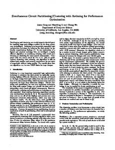
Fig. 2. Comparison of a (blue) simulated eye (218 bits) and a (red) calculated worst case eye. Denoted are eye aperture (EA) and dynamic range (DR) of the eye.
Power estimate(BER) ≤ BERdesired estimate(Area) ≤ Areadesired circuit biasing constraints
where power and area estimates come from transistor-level circuit models, while the bit error rate (BER) is estimated at the system level. This joint formulation captures the interactions in which the system-level parameters depend on circuits, and also the ”circuit biasing constraints” depend on both ”internal” circuit constraints and ”outside/environment” operating conditions set by the system parameters. III. S YSTEM LEVEL MODEL In Figure 1 we show a block diagram of a typical HSL with the signal processing chain (the transmit-equalizer, the channel, the receive-equalizer filters and the slicer decision circuit), and the timing sub-system. The BER constraint of an HSL can be expressed as dmin [k] − RXSens BER = Q( ) < BERdesired σT ot (1) −1 dmin [k] > RXSens + σT ot Q (BERdesired ) where dmin [k] is the minimum distance between the signal constellation points sampled at phase k and the nearest threshold, and σT ot is the aggregate rms value of noise, jitter and residual ISI approximated with Gaussian distribution, BERdesired is the link target BER, and RXSens is the input sensitivity of the decision circuit. To improve the accuracy of the BER estimate for BERdesired < 10−15 (often required in HSLs), the contribution of the residual ISI can be balanced by allocating the N most significant symbol-spaced taps of the symbol response (SR) to the dmin and smaller components to σT ot [14]. In that scenario, dmin [k] can be expressed as the sample under worst case destructive interference [15] at the slicer input for a given sampling phase k, and a subset of N most significant symbol-spaced SR taps aligned with phase k dmin [k] = hk −
n−1 X
j=0, j6=k, mod(j−k,ovsRate)=0
n = N (ovsRate)
|hj |
where hk is oversampled equalized SR and ovsRate is the oversampling rate relative to the link symbol-rate. All remaining SR taps (such as long tails due to reflections at impedance discontinuities) should be treated as additional uncorrelated noise source with rms value of σISI 2 2 2 σT2 ot = σnoise + σjitterV + σISI
(3)
where σnoise is the rms value of the thermal and σjitterV is the rms value of the jitter-induced voltage noise at the receiver [2], [3]. Since the residual ISI dominates the other noise sources in HSLs by an order of magnitude [1], [2], in this work we focus on the optimization of the link signal-processing chain (transmit equalizer and driver, channel, receiver peaking amplifier), noting that the framework can be readily extended to the timing sub-system by using existing jitter-induced voltage noise models [2], [3] and PLL optimization formulations [8]. In Figure 2 we illustrate the values of dmin [k] (i.e. the samples that define the eye aperture) along with the dynamic range of the signal DR, calculated from the SR tap values (4). Dynamic range formulation at the system level ensures proper biasing of underlying transmitter and receiver circuits. dk =
n−1 X
|hj |
j=0, mod(j−k,ovsRate)=0
(4)
DR = max dk k
Since HSLs are usually designed to operate over a range of channels, the link can be simultaneously optimized for a number of channels by adding the constraints (1) and (4) for every channel of interest. The solver performance scales well since increasing the number of constraints in an optimization problem does not significantly affect the performance of interior-point solvers [10]. A. System blocks
(2)
In order to formulate (1) and (4) in terms of link block parameters, we first need to obtain the parameterized transfer function of each signal-chain block in Figure 1. 1) The channel: Figure 3 illustrates the frequency response and binary pulse-amplitude modulated SR at 6.25Gb/s of a typical 32 inch HSL channel. We represent the channel as an FIR filter C(z) =
X
ck z −k
(5)
where ck are impulse response samples of the channel. 2) Transmit-driver/equalizer (T xEq): Transmit-driver provides impedance matching and power gain to drive the channel while the FIR filter provides adequate equalization to ameliorate severe ISI in HSL channels. Table I describes the T xEq system level parameters. Fig. 1.
System level model of a HSL
315
TABLE I T RANSMIT EQUALIZER (T X EQ) SYSTEM LEVEL VARIABLES variable name FIR filter coefficients output swing
variable symbol [1 aF R1 aF R2 . . . ] swingIN
overdrive needed for making a proper decision at a given data rate3 . TABLE III S LICER SYSTEM LEVEL VARIABLES
description equalizer coefficients maximum transmit swing
variable name input noise sensitivity
Transmit FIR operates per-symbol and our formulation works with oversampled symbol response, so we upsample the transmit equalizer response and apply a zero-order hold as in (6). txEQ(z; swingIN, aFR)) = s−1 swingIN X P aF Rdiv(j,
|aF Rk |
ovsRate)
z −j
(6)
j=0
where div(a, b) is integer division. P We normalize the T xEq transfer function in (6) with ||aF R||1 = |aF Rk | to satisfy the output swing limit, since it is convenient to work with aF R0 = 11 . 3) Receiver equalizer (RxEq): To mitigate ISI, peaking amplifiers [17] are often used in HSL receivers along with decision feedback (DFE) equalizers. The system level parameters of an example peaking RxEq are shown in Table II. TABLE II E XAMPLE RECEIVE EQUALIZER (R X EQ) SYSTEM LEVEL VARIABLES variable name gain
variable symbol scale
zero
zRX
drain pole
dpRX
source pole
spRX
description equivalent Z-domain gain of the system coefficient next to the z −1 in the numerator of the transfer function inverse of the pole formed in the drain (in digital domain) inverse of the pole formed in the source (in digital domain)
A discrete transfer function approximation is derived2 as rxEQ(z; scale, zRX, spRX, dpRX) = scale .
1 − zRXz −1 (1 − spRXz −1 )(1 − dpRXz −1 )
(7)
4) Slicer: The slicer system level model is presented in Table III. The sensitivity includes residual offset from process variations and 1 Since
GP-derived solver cannot handle negative optimization variables we use a standard linear programming (LP) trick and express each variable of unknown sign as the difference of two positive optimization variables [16]. Absolute value of an expression can be obtained by upper and lower bounding with a variable [16]. These transformations are used for aF R equalization coefficients and hk SR samples, at the system level. 2 The discretization will be described in further sections with circuit models.
variable symbol σT ot RXSens
description input referred noise of this block input signal needed for resolving
IV. S YSTEM LEVEL FORMULATION With models developed in previous section, and imposed linearity constraints at the circuit level, the HSL system-level model can be represented as a parameterized filter p(z; p) h(z; p) = txEQ(z; p)C(z)rxEQ(z; p) = q(z; p) h(z; p) =
n−1 X
hk (p)z −k ,
p(z; p) =
k=0
s−1 X j=0
q(z, p) =
r−1 X
pj (p)z −j
(8)
qj (p)z −j
j=0
where p = (swingIN, aF R, scale, zRX, spRX, dpRX) is the system level parameter vector. Equation (8) is a parameterized Zdomain representation of the equalized SR used in (2) and (4). Next we need to transform the parameterized transfer function (8) into parameterized SR samples in (2) and obtain the BER constraint (1) from (2). This parameterized SR expression has to perform well in parsing and solving and it has to be easy to generate automatically due to large number of equations. Starting from standard time-domain representation of parameterized SR, we first illustrate the dimensionality issues and impracticality of standard time-domain and direct Inverse Discrete Fourier Transform (IDFT) formulations, and present a set of transformations that lead to a very efficient optimization problem formulation that enables orders of magnitude faster parsing and solving, and real-time joint system-and-circuit optimization. 5) Time domain representation: In order to produce signomial equations describing the equalized SR we can first approximate the IIR filters in (8) with FIR filters. For example, we can use Maclaurin series p(z; p) ≈ p(z; p)˜ q (z; p) (9) q(z; p) where q˜(z; p) = q˜k (p)z −k is an FIR approximation of the IIR filter 1/q(z; p). This approach results in a parameterized expression of each sample of the SR
P
hk (p) =
n−1 X
pj (p)˜ qk−j (p)
(10)
j=0
While this formulation is optimizer-compliant and performs well on smaller problems, it is very limited in practical HSL channels due to its size. An example HSL formulation quickly reveals this curse of dimensionality: • channel impulse response samples: 20 (bit-spaced) st • IIR filters: 2 filters, 1 order each • IIR expansion terms: 15 (gives accuracy of 3% for typical pole locations) • oversampling: 10 (relatively low) (a) Typical symbol-spaced binary NRZ (b) Typical transfer function magniSR of a channel at 6.25Gb/s tude Fig. 3.
A 32 inch off-chip interconnect example
3 Overdrive is inversely proportional to the slicer gain which is an exponential function of the symbol time due to positive feedback in the decision circuit.
316
since the parameterized SR expression has (20 × 10) × (15 × 10)2 = 4, 500, 000 terms. The SR is (20 × 10) + (15 × 10) + (15 × 10) = 500 samples long, where each sample consists of many terms. This example is a bit optimistic, since our link model should have at least 2 IIR filters and 2 FIR filters. With this complexity of expressions the time to generate the system level description as well as the parsing time are on the order of days, even for this simple example, rendering this approach impractical. 6) Direct IDFT: The next logical approach to formulating the system level is to directly manipulate the expressions in Z-domain. Calculating the overall SR from (8) is done by performing IDFT in n points z0 , . . . , zn−1 on the unity circle in Z-plane n−1
hk (p) =
1 X p(zj ; p) j z , n q(zj ; p) k
k = 0, . . . , n − 1
(11)
j=0
which has fewer terms than (9) and is much easier to generate. However, it is not very efficient in parsing time and has issues with numerical stability. Rational expressions require a large number of operations in the parser to generate the signomial form. In terms of the calculation in the previous section, for this approach we would have n = 500, and each of these 500 equations contains all of the 500 hk we wish to recover. Thus, system is represented with a 500 × 500 dense matrix. 7) Solution - Indirect IDFT: The previous two formulations were trying to obtain an expression for each sample of the equalized SR. While very natural from designer’s perspective, this approach creates very complicated and long expressions with large number of terms. The optimization-based flow offers the possibility to do better by taking a different perspective. This is the central point of our work as we show that both system and circuit level can be designed jointly using existing circuit optimization technology. This different approach turns the SR formulation into a fitting problem. We give up on the idea of finding exact expression for each sample separately, but try to come up with a set of simpler equations whose solution is exactly the needed SR. In particular the SR samples in our formulation are, from now on, defined as optimization variables and not closed-form expressions, hk (p) → hk . Furthermore, we wish to avoid numerical problems linked to rational expressions. To implement these ideas we rewrite (11) and (8) as E(z; p, h) = q(z; p)
n−1 X
hk z
−k
− p(z; p)
(12)
k=0
where p(z; p) and q(z; p) are parameterized filters. We can interpret E(z; p, h) as the fitting error in the Z-domain. With this in mind we impose the following set of constraints in the formulation −tol ≤ E(zj ; p, h) ≤ tol,
j = 0, . . . , n − 1
(13)
where we can perform tradeoff between the fit accuracy and solution time with with tol → 0. The obtained formulation (13) is compact and can be generated and parsed quickly. However, it requires long time to solve since each equation contains all the optimization variables4 . To avoid this we need to perform one more transformation step before passing the formulation to the solver.
We see that, in (12), it is possible to perform multiplication of q(z; p)h(z), which has the same effect as convolution of coefficients in q(z; p) and h(z). Furthermore, we can represent the fitting error in frequency domain as a sequence of error samples in time, thus arriving to n+r−1
X
k=0 n+r−1
X
=
r−1 X
qi (p)hk−i
i=0
k=0
!
(14) z
−k
− p(z; p)
with deg(z, p(z; p)) ≤ n which is always satisfied. The most important point in our derivation of the system level formulation is to note, in (14), that for HSLs r = deg(z, q(z; p)) V in cm > V in min
% system variable linking system.swingIN = txEQ.swingIN; system.zRX = rxEQ.zRX;
IHI = 1.8M1 tail .ids ILO = 0.2M1 tail .ids M1 hi.ids ≤ IHI M1 lo.ids = 2M1 .ids − M1 hi.ids statP = 2Vdd M1 tail .ids
···
% operating conditions rxEQ.max Vin ≥ txEQ.comm mode + system.DR; xEQ.min Vin ≥ txEQ.comm mode - system.DR;
we used instances M1 hi and M1 lo to represent input transistor (M1 ) in different operating conditions when signal at its gate achieves maximum and minimum value. We assumed that we can, at most, switch between 20% and 80% of the total bias current, which is M1 tail .ids + M2 tail .ids = 2M1 tail .ids = 2M1 .ids. Finally, we discretize this analog filter transfer function to fit in our system level formulation, using Tustin’s transform6 1 + ωz2Ts vout g m Ts (z) = h(z) ω vin CD 2 (1 + pd Ts )(1 + ωps Ts ) 2
2
1− h(z) = (1 + z −1 ) (1 −
ωpd Ts 1− 2 ωpd Ts 1+ 2
ω T 1− z2 s ω T 1+ z2 s
z −1
z −1 )(1 −
1− 1+
(22) ωps Ts 2 ωps Ts 2
dpRX1 =
1 + ωz2Ts ωpd Ts ω T )(1 + ps2 s ) 2 1 − ωz2Ts 1 + ωz2Ts ω T 1 − ps2 s spRX1 = ω T 1 + ps2 s
g m Ts CD 2 (1 +
1− 1+
ωpd Ts 2 ωpd Ts 2
,
(24) .
C. Predriver/Slicer/DFE The predriver, slicer and DFE are currently included as placeholders, with defined interface variables. For example, predriver 6 We choose this transformation due to the mapping between analog and . digital domains that can be expressed in signomial form s = T2 z−1 z+1 s
Fig. 5.
Capacitively peaked receiver equalizer
2system.dmin [k] ≥ slicer.sensitivity + (slicer.sigma)(Q(1e-15));
% objective min: txPredriver.power + txEQ.power + rxEQ.power + slicer.power;
power is estimated according to the driver input capacitance and fan-out sizing rules that depend on the link data-rate. Similarly, the slicer is currently abstracted through its input biasing requirements and system-level sensitivity and noise variables. While modeling of any link circuit requires careful consideration, we do not foresee significant difficulties in including more accurate circuit models for these blocks in our optimization flow. VI. P UTTING EVERYTHING TOGETHER
(23) ωps = (1 + gm RS )/τS , ωpd = 1/τD We take into account the parasitic capacitance in the drain of M1/2 in CD along with Cp from Figure 5. We can finally link the circuit parameters to the system level parameters we defined in Table II
zRX1 =
% performance
z −1 )
and time constants of the model can be defined as τS = RS CS , τD = RD CD , ωz = 1/τS
scale =
···
With all the modules in place, and defined interface variables, the last step is to formally link all of them. In our example this is done by instantiating all the necessary models as sub-blocks (in this way even the system level formulation becomes a sub-block), Listing 5. Then we simply impose equality constraints between appropriate interface variables, which is made easy by the signomial-based formulation. We also link operating conditions of each circuit to the overall system settings at this level. Finally, the sampling phase has to be chosen at which we specify the BER constraint (1). In a sense, we can think of our system level formulation as a specification setting layer. For any change in transmit equalization it will readjust the input dynamic range into the receiver equalizer as well as recalculate the eye aperture thus changing the specifications of the receiver, and vice versa. We can see this, for example, in Listing 5 in sections on operating conditions where input dynamic range of the peaking amplifier is adjusted according to system level estimate of the dynamic range of the signal at its input (4). This is exactly where the iterative loop of the traditional design flow is replaced. A. Results To test our formulation we try to design an HSL system communicating over a 32 inch channel with transfer function given in Fig. 3(b). Our objective is power minimization while requiring that dmin [k] ≥ 50mV . In our circuit formulations we used signomial and posynomial transistor models extracted from predictive 90nm technology models. The trade-off between link power and sampling phase is shown in Fig. 6(a) indicating a significant dependence on the sampling position and offering the possibilities for efficient exploration of equalization and CDR interaction. By running the formulation at multiple data rates and picking the instances with best power results we can see how the system power scales with data rate, Fig. 6(b). We run optimizations for 4Gb/s,
319
(a) Power vs. sampling phase for 6.25Gb/s, no DFE
Fig. 7. Accuracy of calculated symbol response using formulation (16) against Matlab calculation
(b) Power vs. symbol-rate Fig. 6.
Dependency of power on symbol rate and sampling phase
6.25Gb/s, 8Gb/s and 10Gb/s, Table IV. The results suggest that dmin [k] ≥ 50mV constraint is achievable at 8Gb/s only with 1-tap DFE and at 10Gb/s we could only achieve dmin [k] ≥ 35mV even with 4-tap DFE. Here, the DFE assumption is introduced only at the system level, by omitting certain number of post-cursors from the dmin [k] equation (2). This means that the overall power numbers for 8Gb/s and 10Gb/s are optimistic. On the receiver side, the analog peaking amplifier consumes around 5% − 10% of power at lower speeds and between 20%−30% as we keep increasing the speed. It is interesting to see that, for the given link topology, no solution actually had significant peaking in the RxEq. In all our design attempts, the best solution was using wideband analog receiver amplifier in RxEq with the bandwidth always above the Nyquist frequency. Since this choice defies conventional wisdom, we further investigate this result in more detail. In the first column of Table IV we show the results of an optimization-run without any transmit side equalization, where the receive peaking amplifier takes on the role of the equalizer. Note that in this situation, RxEq is forced to provide high-frequency gain under large input dynamic range, which requires a lot of power. Since in capacitively peaked amplifier, peaking is achieved by lowering the DC gain and higher overall system power than in the case where T xEq and receive amplifier are used (second column of Table IV), Figure 6(b). In the case with no T xEq the system compensates for the decrease of RxEq DC gain by increasing TABLE IV S OME OPTIMIZATION RESULTS rate [Gb/s] swingIN [mV] aFR RxEq gain ωz /(2π) [GHz] ωdp /(2π) [GHz] ωsp /(2π) [GHz]
4 200 none 1.1 0.8 2.1 2.6
4 100
h
1 −.42 3.5 2.4 3.4 5.4
6.25 200
i
h
8 280
i
1 −.52 2.7 4.7 5.7 5.8
"
10 330
#
1 −.42 −.05 2.1 2.2 3.6 10
"
#
1 −.43 −.15 3.3 3.4 3.6 3.3
the transmit side swing. This interaction shows that our system level formulation does in fact manage to express tight inter-dependencies between system blocks that optimization engine can utilize. For a designer who is just focused on the block level, these interactions are hard to capture. Looking further in the table, we can observe that from 4Gb/s to 6.25Gb/s optimizer chooses to apply more aggressive equalization at the transmitter. This is expected, as the channel has stronger postcursors at 6.25Gb/s and more equalization is needed. However, this trend does not continue through 8Gb/s and 10Gb/s cases, since at these data rates the channel attenuation is so high that only DFE can meet the BER requirements. Since in our setup, the optimizer does not see any penalty to utilizing DFE (no circuit model is supplied, thus no power increase is observed) it performs most of the equalization with DFE. The T xEq is still utilized to control the peak-to-average ratio of the signal entering the receive amplifier due to our constraint on input dynamic range of this circuit in order to preserve linearity. We see that transmit equalizer can be used for equalization purposes in order to achieve better eye aperture, but also as a means to control operating conditions of the receive amplifier. In short, our results indicate that interaction between different methods of equalization could be studied through the developed framework. B. Verification Finally, we check the accuracy of our formulation method when compared to the standard tools used in HSL design. In Fig. 7 we compare symbol response for one of the cases discussed (optimal sampling phase for 6.25Gb/s) obtained in our optimization formulation against appropriate Matlab calculated response for the same equalization settings. We see exceptional matching between these waveforms with less than 2mV of absolute error ek . This can be further improved by tightening optimizer parameters with solution time penalty as we noted in reference to (13). Finally, we run Spectre simulations for the design obtained for 6.25Gb/s presented in Table IV to confirm proper biasing and performance of the T xEq and RxEq circuit blocks. We found that transistor biasing was done properly to the 10 − 30% accuracy in terms of saturation voltages. T xEq and RxEq parameters (output swing, gains, poles and zeros) were all matched to within 10%7 . 7 The AC pole-zero analysis in Spectre revealed that source impedanceinduced pole and zero of the RxEq require better modeling due to the neglected positive feedback through output conductance gds of the input transistors M1/2 . With appropriate correction our results match the simulation well.
320
C. Computational efficiency We tested our design flow by running design optimizations for the channel in Figure 3 at 4Gb/s, 6.25Gb/s, 8Gb/s and 10Gb/s. The system formulation dominated the size of the whole formulation in terms of the number of different optimization variables and optimization constraints. Thus the parsing and solution time were mostly due to the system level formulation. In general, our problems had between 1500 and 1700 variables and between 4500 and 5500 constraints, depending on the actual number of significant samples in the SR, which changes with data rate. In terms of run time, the developed flow is very efficient. Our optimization runs were executed on a laptop with 1.60GHz Pentium M processor and 2GB of memory running Debian Linux. The parsing time varied between 15 minutes and 1 hour, while the solver time was between 1 hour and 3 hours. The overall solution time was below 4 hours for any of the configurations. The developed formulation is a very efficient tool for design space exploration. It is well-suited for design of such complicated systems as HSLs over multiple channels and process corners. With appropriate formulation and circuit model adjustments it could be applied to any mixed signal front-end design. VII. C ONCLUSIONS Design of power-constrained analog/mixed-signal front-ends, especially radios and high-speed links requires careful balance of power allocation among the circuits in the signal chain. In traditional iterative design approach, the system performance modeling and circuit design are rather disjoint or at best connected in an ad-hoc manner. By casting the high-speed link performance model as a symbolic signal transformation problem, with filters parameterized by circuit performance properties, we were able to establish an efficient problem formulation for joint system-and-circuit optimization. This efficient formulation improves the tractability of the optimization by several orders of magnitude and enables real-time optimization. We illustrated the potential of this framework on a simplified high-speed link example, showing the potential of the new formulation. Although quite simplistic, this example allowed us to address for the first time the possible trade-offs between transmit and receive equalizers in a unified manner, showing the mechanism through which they interact with channel loss and other circuit constraints like input and output dynamic range. To the best of our knowledge, this is the first work to introduce transistor level circuit models in system level design of an HSL by means of optimization. VIII. ACKNOWLEDGMENTS We are grateful to the people of Sabio Labs: Mar Hershenson, Sunderarajan Mohan, Dave Colleran, Almir Mutapˇ ci´c and Shyne Tseng for all their useful hints, discussions and support in terms of Sabio software environment and debugging experience. We would also like to thank Mosek for providing us with their high quality optimization solvers. This work was supported by the Center for Integrated Circuits and Systems at MIT and in part by Lincoln Laboratories Advanced Concepts Committee.
[3] P. Hanumolu, B. Casper, R. Mooney, G.-Y. Wei, and U.-K. Moon, “Analysis of pll clock jitter in high-speed serial links,” IEEE Transactions on Circuits and Systems II: Analog and Digital Signal Processing, vol. 50, no. 11 SN - 1057-7130, pp. 879–886, 2003. [4] H. Hatamkhani and C. Ken Yang, “A study of the optimal data rate for minimum power of i/os,” IEEE Transactions on Circuits and Systems II, vol. 53, no. 11 SN - 1057-7130, pp. 1230–1234, 2006. [5] M. Hershenson, S. Boyd, and T. Lee, “Optimal design of a cmos op-amp via geometric programming,” IEEE Transactions on Computer-Aided Design of Integrated Circuits and Systems, vol. 20, no. 1 SN - 02780070, pp. 1–21, 2001. [6] P. Mandal and V. Visvanathan, “Cmos op-amp sizing using a geometric programming formulation,” IEEE Transactions on Computer-Aided Design of Integrated Circuits and Systems, vol. 20, no. 1, pp. 22–38, 2001. [7] M. del Mar Hershenson, “Design of pipeline analog-to-digital converters via geometric programming,” in ICCAD ’02: Proceedings of the 2002 IEEE/ACM international conference on Computer-aided design, 2002, pp. 317–324. [8] D. Colleran, C. Portmann, A. Hassibi, C. Crusius, S. Mohan, S. Boyd, T. Lee, and M. del Mar Hershenson, “Optimization of phase-locked loop circuits via geometric programming,” Proceedings of the IEEE Custom Integrated Circuits Conference, 2003., no. SN -, pp. 377–380, 2003. [9] X. Li, J. Wang, L. Pileggi, T.-S. Chen, and W. Chiang, “Performancecentering optimization for system-level analog design exploration,” in IEEE/ACM International Conference on Computer Aided Design (ICCAD), 2005, pp. 422–429. [10] S. P. Boyd and L. Vandenberghe, Convex Optimization. Cambridge, UK: Cambridge University Press, 2004. [11] C. Maranas and C. Floudas, “Global optimization in generalized geometric programming,” pp. 351–370, 1997. [12] J. Kim, J. Lee, L. Vandenberghe, and C. Yang, “Techniques for improving the accuracy of geometric-programming based analog circuit design optimization,” IEEE/ACM International Conference on Computer Aided Design (ICCAD), no. SN - 1092-3152, pp. 863–870, 2004. [13] W. Daems, G. Gielen, and W. Sansen, “Simulation-based automatic generation of signomial and posynomial performance models for analog integrated circuit sizing,” IEEE/ACM International Conference on Computer Aided Design (ICCAD), no. SN -, pp. 70–74, 2001. [14] V. Stojanovic, A. Amirkhany, and M. Horowitz, “Optimal linear precoding with theoretical and practical data rates in high-speed seriallink backplane communication,” IEEE International Conference on Communications, vol. 5, no. SN -, pp. 2799–2806 Vol.5, 2004. [15] J. Ren and M. Greenstreet, “A unified optimization framework for equalization filter synthesis,” in DAC ’05: Proceedings of the 42nd annual conference on Design automation, 2005, pp. 638–643. [16] D. Bertsimas and J. N. Tsitsiklis, Introduction to Linear Programming. Athena Scientific, 1997. [17] R. Farjad-Rad, N. Hiok-Taiq, M. Edward Lee, R. Senthinathan, W. Dally, A. Nguyen, R. Rathi, J. Poulton, J. Edmondson, J. Tran, and H. Yazdanmehr, “0.622-8.0 gbps 150 mw serial io macrocell with fully flexible preemphasis and equalization,” Symposium on VLSI Circuits, 2003. Digest of Technical Papers. 2003, no. SN -, pp. 63–66, 2003. [18] J. Zerbe, C. Werner, V. Stojanovic, F. Chen, J. Wei, G. Tsang, D. Kim, W. Stonecypher, A. Ho, T. Thrush, R. Kollipara, M. Horowitz, and K. Donnelly, “Equalization and clock recovery for a 2.5-10-gb/s 2pam/4-pam backplane transceiver cell,” IEEE Journal of Solid-State Circuits, vol. 38, no. 12 SN - 0018-9200, pp. 2121–2130, 2003.
R EFERENCES [1] B. Casper, M. Haycock, and R. Mooney, “An accurate and efficient analysis method for multi-gb/s chip-to-chip signaling schemes,” Symposium on VLSI Circuits Digest of Technical Papers, 2002., no. SN -, pp. 54–57, 2002. [2] V. Stojanovic and M. Horowitz, “Modeling and analysis of high-speed links,” in IEEE Custom Integrated Circuits Conference, 2003.
321