concentrates on the solution methodology for pumped-storage units. A pumped-storage unit can be operated in generation, pumping or idle slates. It can smooth ...
IEEE Transactions on Power Systems, Vol. 9,No. 2,May 1994
1023
Optimization-Based Scheduling of Hydrothermal Power Systems with Pumped-Storage Units
Xiaohong Guan, Peter B. Luh, Houzhong Yan J3cpt. of Elec. & Syst. Engineering University of Connecticut StoiTS, CT 06269-3157, U.S.A.
Abstract. This pipei presents an optimimtion-based method for scheduling liydrollrerinal systems based on the Lagrangian relaxation technique. After system-wide constraints are relaxed by Lagrange multipliers, the problem is converted into the scheduling of individual units. This paper concentrates on the solution methodology for pumped-storage units. A pumped-storage unit can be operated in generation, pumping or idle slates. It can smooth peak loads and provide reserve, therefore plays an impoi tan1 role in ieducing total generation costs. There are, however, many constraints liniiting the operation of a pumped-storage unit, such as pond lcvel dynamics and constraints, and discontinuous generation and pumping legions. Moreover, according to the current practice, the dynamic transilioiis among operating states (generation, pumping and idle) Ne not arbitrary. The most challenging issue in solving pumpedctoiage subproblems within the Lagrangian relaxation framework is the inlegiated consideration of these constraints. The basic idea of our method is to relax the pond level dynP )
1
I.k(t) =
T
+ I f ; [ w p d ( t+ ) Pl(t)Pl(f)J>
(3.7)
= 1 , 2,......, T .
(3.8)
subject to p(t) 20,
t
3.2 Quadratic Approximation of the Water-Power Conversion Function Since ppk(wk(t))is piece-wise linear with respect Lo W k ( t ) as shown in Fig. 2 and r P k ( p p k ( w k ( t ) ) ) is piece-wise h e a r with respect Lo ppk(wk(t))as shown in Fig. 3, Lpk(wk(t)) in (3.6) is a piece-wise linear function of w k ( t ) with coefficients determined by Lagrangian multipliers. When the pond level limit in (2.5) is not active, tlie optimal generation or pumping is generally obtained at one of the comer or boundary points: maximum generation/pumping. minimum generatiodpwnping, maximum . . - therefore reserve or idle (zero). The optimal generation or pumping changes from m e of these points to another as the multipliers change, This sohilion oscillation lndy lead to numerical instability. To overcome this dilliculty, a quadlatic function is used to approximate the water( ~ ) )then be power conversion as shown in Fig 4. The power J J ~ ~ ( M ’ ~ will a quadratic iunction of w k ( t ) , and this in turn leads to a piece-wise quadlatic L P k ( w k ( t ) ) .The optimal generation or pumping (herefore no longer jumps from one comer point to another over the iteiations, and the diflicnlties caused by solution oscillation can be avoided. To differentiate from the original water-power conversion, the new conversion is denoted as ] j y k ( W t ) ) , new cost as i p k and new subpioblem as (Yp-k-).
3.3 Solving Pumped Storage Subproblems Given /z and p, the pumped-storage subproblem (fp-k)is to determine the generation or pumping at each hour so as to minimize the cost funclion (3.6) subject lo individual constraints (2.4)-(2.12) and operating slate dynamics. Although this cost function is stage-wise additive, the generation or pumping at hour t cannot be determined by simply minimizing the stage-wise cost function at that hour since pond level constraints (2.4)-(2.6) couple decisions across hours. Furthermore, operating regions
(3.9)
By substituting the above equation into the pond level limit9 and terminal condition (2.5)-(2.6), the pond level dynamics and constraints can be rewritten as f
v; - c, In=z1w k ( n ) I ; V ; ,
To obtain a new optimal solillion, efficient algorithms are needed
for solvulg three lypes of subproblems, solving tlie dual problem, and also for constructing a feasible solution.
vi - n=l c Wk(12).
t = 1,...,T - I ,
(3.10)
and
$ )1‘k(n) = v i - vi.
(3.11)
n=l
By using additional sets of multipliers B k , (3.11), the cost function in (3.6) becomes:
yk
and