Optimization Models for Designing Aggregation

Optimization Models for Designing Aggregation Networks to Support Fast Moving Users Frederic Van Quickenborne, Filip De Greve, Ingrid Moerman, Filip De Turck, Piet Demeester Department of Information Technology (INTEC) Ghent University - IMEC Sint-Pietersnieuwstraat 41, B-9000 Gent, Belgium. Tel.: +32 9 264 99 57, Fax: +32 9 264 99 60 {Frederic.VanQuickenborne, Filip.DeGreve}@intec.ugent.be

Abstract. In this paper, the focus is on the design of an aggregation network for offering high-bandwidth services to fast moving users (e.g., users in trains or cars). The overall considered network architecture consists of two parts: an access network part and an aggregation network part. The users in the fast moving vehicles are connected to the access network via a wireless connection. In the aggregation part, traffic of different users is bundled together in tunnels, and as the users move from one access network to access network, tunnels have to move with them. Two problems concerning this issue are tackled in this paper. The first one can be described as follows: how to determine the tunnel paths in the aggregation network to meet the fast moving traffic demand of requests while achieving low congestion and minimizing the network dimensioning cost. Secondly we need protocols to manage the tunnels by means of configuration and activation at their due time. GVRP (GARP (Generic Attribute Registration Protocol) VLAN Registration Protocol) and a new GARP protocol, called G2RP, were designed and implemented as protocols for the automatic tunnel configuration and activation, respectively. Finally, the performance of the different algorithms used for the network capacity planning and the tunnel path determination will be compared on basic train scenarios. Keywords Capacity assignment, traffic engineering, mobility support

1

Introduction

Nowadays, a lot of multimedia applications are taken for granted in fixed networks. These applications, such as managed home networking, multimedia content delivery, video phoning and on-line gaming require a high level of Quality of Service and are generally characterized by high bandwidth requirements. Current telecom-operators have mainly designed their broadband networks to cope with rather static or slowly evolving traffic demands while fast moving traffic conditions have never been taken into account. The challenge is to design telecom networks in such a way that high bandwidth services can be provided to

Required Bandwidth 1 Gbit/s

Tunnel management

Tunnel Tunnel Tunnel 1 2 3

GVRP: automatic establishment of tunnel path, found by tunnel path determination algorithm, without reserving the required resources

time t1

t2

t3

G2RP: automatic activation of the configured tunnels at their due time, and de-activation when they are not needed anymore

SGW Service Provider Domain

0 AGW

GVRP

6

G2RP

1 t1

Tunnel 1

Aggregation Network

Ethernet Switch 5

Tunnel 2 Tunnel 3 Access Network 2

3

t2

4

t3

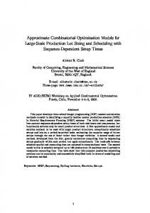
Fig. 1. Schematic representation of considered network architecture, which consists of an access part and aggregation part. The designed protocols for tunnel configuration and tunnel activation are shown as well.

fast moving users (e.g., in the car or on the train). These networks can typically be deployed in metropolitan areas, along railroad tracks or along highways. For an example of such a network, the reader is kindly referred to [1]. The considered network architecture in our paper is depicted in figure 1. As can be seen in this figure, the architecture is divided in an access network part and an aggregation network part. The main difference between these two parts is that in the access network part, traffic demands from separate users are considered, whereas in the aggregation network part, groups of users are aggregated together. We define one or more groups of users per train. The traffic of each group of moving users is multiplexed in the Access Gateways (AGWs) into a tunnel. These AGWs provide the connections between the access network and the aggregation network. The aggregation of the groups is done by taking the users together in tunnels in the aggregation network, as depicted in figure 1. In this figure we consider three time-events: t1 , t2 and t3 on which the train is

connected to three different access networks. The total required bandwidth for the train is 1 Gbit/s, based on a calculation made in [2]. On t1 , Tunnel 1 is used to meet the traffic demand of the train. On t2 , Tunnel 2 is used, and on t3 , Tunnel 3. The aggregation network is responsible for the transport of aggregated data traffic, by means of high bandwidth tunnels moving at high speed, between the access networks and service provider (SP) domain such as Internet service providers (ISPs), content providers and telephony operators. The connection between the SPs and the aggregation network is realized by Service Gateways (SGWs). The fast moving aspect of the traffic demands (leading to rapidly moving tunnels) has not been extensively studied for aggregation networks. E.g., a detailed description of the UMTS technology in [3] gives only a brief description of the used protocols for interaction with the fixed network. The main problem, tackled in the paper, can be described as follows: how to calculate and set up dynamic tunnels between the gateways in the aggregation network to meet the traffic demand of requests while achieving low congestion and optimizing the utilization of the network resources. In order to automatically invoke the set-up of the required tunnels and activate the tunnels at their due time, protocols are required. Two different protocols are designed for handling the tunnel configuration and activation requests. But first the optimal path for each tunnel needs to be determined. Therefor a theoretical network capacity planning and dimensioning model is implemented that optimizes the use of resources under rapidly moving but quite predictable traffic conditions. Due to the complexity of the problem, rigorous optimization by means of ILP (Integer Linear Programming [4]) techniques only delivers solutions in a reasonable calculation times for limited network sizes. Therefore, we present several approaches to shorten the solution times. The model also includes a path calculation algorithm that is specifically designed for fast moving user conditions. Mainly for economical reasons telecom operators [5] tend towards networks consisting of standard QoS-aware Ethernet switches (IEEE 802.1d [6], IEEE 802.1q [7] & p, IEEE 802.1s [8] compliant). We do not consider satellite or UMTS technology, due to their respective limitations of latency and bandwidth for fast moving users. The protocols for tunnel configuration and activation are implemented for Ethernet aggregation networks. The designed protocols allow to make optimal use of VLANs (Virtual LANs [7]) to support Multiple Spanning Trees in the Switched Ethernet networks. In this way network resources are optimally used. The reader is referred to 2.1 and 2.2 for a description of the VLAN tunnel set-up mechanisms. The remainder of this paper is structured as follows: section 2 describes the self designed and implemented protocols for tunnel configuration and tunnel activation and section 3 details the implemented model for optimal network capacity planning and tunnel path determination. Section 5 considers the evaluation results. In the final part of the paper in section 6, some interesting conclusions are summed up.

2

Tunnel configuration and activation

Based on the determined optimal path for each tunnel, found by the solution method described in section 3, the tunnels are configured in the network by means of GVRP (GARP (Generic Attribute Registration Protocol) VLAN Registration Protocol). At activation time the resource reservation is done by means of the G2RP (GARP Reservation Parameters Registration Protocol) protocol. This section gives a brief operational description of both protocols. For an extensive description, the reader is kindly referred to [9], which also contains extensive performance measurements of both protocols. 2.1

GVRP

Based on the output of the network dimensioning process, the paths for each required tunnel are calculated. The path calculation aims at minimizing the total resource usage by applying optimization algorithms, which are detailed in the next section. Based on the determined path for each tunnel, these tunnel are configured in the network by means of GVRP (GARP (Generic Attribute Registration Protocol) VLAN Registration Protocol). This protocol automatically establishes the tunnel path, without reserving the required resources. It is a GARP compatible protocol (standardized by IEEE 802.1q [7]) and sets up the tunnel path by means of automatic VLAN registration on every switch of the network. Due to the fact that GVRP was initially not designed for a VLAN tunnel, but rather for a sub-tree of the topology, the protocol suffers from a lot of overhead registrations. To deal with this problem, we developed the ”Scoped Refresh” extension of GVRP. For details of this extension, the reader is again kindly referred to [9]. 2.2

G2RP

The main purpose of this protocol is to activate the configured tunnels at their due time, and de-activate them when they are not needed anymore. Instead of extending GVRP to support propagation of reservation parameters (bandwidth parameters, QoS class, burst size and the size of the time sample window) and activation and de-activation of tunnels, a new GARP protocol is designed. This protocol is called GARP Reservation Parameters Registration Protocol (G2RP). By separating the configuration of tunnels and the distribution of reservation parameters, G2RP remains independent of the applied tunnel configuration mechanism. G2RP is designed according to the GARP standard. G2RP will translate the activation and de-activation triggers into hardware operations. Basically, the switch hardware (bandwidth shapers, classifiers, queues, etc.) will be configured according to the reservation parameters for the associated configured tunnel. Before any activation takes place, G2RP will consult the admission control. Admission control is added to keep track of the existing bandwidth reservations. If at any point along the VLAN tunnel the available hardware resources are not sufficient to support a specific reservation, the activation will fail and this will lead to an error indication.

Simple solution technique detecting shortest path from every AGW to the SGW; cost = 12 interface cards needed for tunnel between SGW and AGW 3

SGW

for tunnel between SGW and AGW 2

for tunnel between SGW and AGW 1

Our solution technique ILP solution technique; cost = 8 interface cards needed or 33% cheaper

AGW 3

2 SGW 1

t'1

t'2

time t'3 events

Fig. 2. Two different solutions for a simple problem: on the left side a simple solution technique that detects the shortest path from every AGW to the SGW and adds those links to the network dimensioning. The solution on the right is the one found by our implemented solution technique. This solution is for this simple example 33% cheaper.

3

Network capacity planning and tunnel path determination

Subsection 3.1 proves the need for a model for optimal network capacity planning and tunnel path determination, while subsections 3.2 and 3.3 details the assumptions concerning the considered network and traffic parameters. A formal definition of the aggregation network capacity planning and related tunnel path determination will be presented in subsection 3.4. Subsection 3.5 details the developed solution technique. 3.1

Why model needed for capacity planning and tunnel path determination?

3.2

Network model

For now, we assume a single service gateway and we assume that successive access gateways are positioned along the railroad track every 7,5 kilometers, based on a calculation made in [2]. Passing trains will connect to the closest access network and will hop from one AGW to another. The SGWs are constantly updated with the current position (and future positions) of the train and updates at every turn the next hop gateway for the IP routing towards the moving user [10]. To optimize the cost of the network we assume the links to be already installed and we only take the node cost into account. We distinguish between different line card types of different speeds and with different port ranges. The model will ensure that link and node capacities are adjusted appropriately. The model allows a large flexibility: removing certain card ranges on nodes, different prices of different hardware vendors can be taken into account. We assume that for

every traffic class a single path is used for routing for every AGW-SGW pair at a certain moment. This path may vary in time but it will always be the same for a traffic class. In other words, this supports that different traffic classes of one train may be routed differently. Traffic demands vary depending on wether the application is symmetric (video conference) or asymmetric (video broadcasting). Both symmetric and asymmetric demands can be taken into account in the proposed model. We define a set of access gateways: AGW = {agwi }, with index i indicating the different access gateways and a set of service gateways: SGW = {sgwk }, with index k indicating the different service gateways. To characterize the network, we define a given set of unidirectional edges: E = {e} and a given set of nodes: N = {n}. In addition we define a set of links: L = {l} with every (bi-directional) link consisting of two unidirectional edges given by set El = {el , e0l } with same source-destination node pair as link l. We like to remark that ∀l : |El | = 2. Each node is characterized by the speed of every interface and the number of interfaces, possibly grouped together on one card (e.g., one card with two Gigabit interfaces): Cv = e.g., {100|1000|10000} , v = 1 . . . |V | ; (1) ∀v : Ovw = e.g., {1|2|4} , w = 1 . . . |Ov | .

(2)

V gives the set of strings, each describing a different type of interface which are present on a node; Cv defines the different speed of every type of the set V, in this example going from 100 Mbit/s to 10 Gbit/s; Ov gives the set of possible configurations of the cards of a certain type, given by v ; more specific, Ovw gives the number of interfaces present on a card for every type of card. 3.3

Traffic model

In order to describe the traffic demands, we define flows j as being the basic routing unit: this allows different levels of abstraction. We can define one flow per train, one flow for every QoS class per train, etc. Traffic loads per AGW are associated with the flows as they move along the AGWs. The traffic demands for the AGWs are represented as a set of signals present at every agwi : Si = {sij (t)} , j = 1 . . . |Si | with index j indicating the different flows. We also define the total number of signals for each agwi : Ji = |Si |. Each train that passes the antennas connected to an AGW results in a certain demand for the specific agw from a specific server: Dik = {dijk (t)} with index i indicating the AGW, k indicating the SGW and j is used to make a difference between the different flows. To indicate if the demand at a certain agw is above zero and thus active, we introduce ( PP 1, if dijk (t) > 0 t k aij = . (3) 0, otherwise Due to the moving aspect of trains, the traffic demands are time dependent. However, the dimensioning problem is not continuous and can be solved for a limited set of discrete events. Therefore, we define a set of events that are

critical for the dimensioning. These events are all the discrete time points when the traffic conditions change. However, this set contains a lot of events which are redundant for the dimensioning problem. In order to minimize the amount of constraints for the dimensioning problem, the set of events is reduced: e.g., for a single AGW scenario, if the network must be able to support a certain demand to this AGW, all the events with lower demands for the AGW (under same other circumstances) are already covered and are removed from the set of events. The set of reduced time events is given by T 0 = {t0 }. 3.4

Problem formulation: network capacity planning and tunnel path determination

1. Variables First of all, the variables of the ILP-problem are defined. The first one represents the number of line cards available in each node: znvw = # of cards with Ovw interfaces of speed Cv on node n.

(4)

Each card has a specific cost, cvw , depending on the speed of the interfaces on the card (Cv ) and the number of interfaces installed on the card (Ovw ). The following parameter gives information about the number of fibres on every link: xvl = # of fibres with speed Cv on link l. (5) With this information, one can calculate the capacity of every link in the network: X Cl = xvl · Cv . (6) v

2. Node capacity constraint Every node needs enough interfaces with appropriate specifications (given by indices v and w ) to provide the links that are connected to it: |Ov |

∀n, ∀v :

X w=1

znvw · Ovw ≥

X

xvl .

(7)

l∈out(n)

Link flow formulation 1. Variables Besides the previous defined variables, we also need a variable to indicate if a certain edge e is used for a certain flow j :  1, if edge e is used between i and k for flow j yeijk = . (8) 0, otherwise

2. Link Capacity constraint This constraint imposes that the traffic that is transported over a link does not exceed the capacity of that particular link: P PPP yel ijk·dijk (t) ≤ xvl · Cv ,  v i P j k P P ∀l, ∀t ∈ T 0 : P (9) ye0l ijk·dijk (t) ≤ xvl · Cv .  k

i

v

j

3. Flow Conservation constraint The last constraint imposes that a flow is not interrupted in the network: P P ∀n, ∀k, ∀i, ∀j : yeijk − yeijk = e∈out(n) e∈inc(n)   anj , if node n is the source for the flow (10) −ain , if node n is the desired agw .  0, otherwise 4. Objective function c c=

v| X X |O X

n

v

w=1

znvw · cvw +

XXXX k

i

j

yeijk · cl · Cj .

(11)

e

The first part is the cost for the network devices in the network while the second part is the routing cost in the network, in which cl gives us the cost for every link and Cj represents the bandwidth of each flow. The aim of the optimization algorithm is to minimize c. Path Flow formulation 1. Variables First we have to define a set of possible paths for each SGW-AGW pair: Pik = {pikq } ,

(12)

in which index q is used to indicate the different considered paths between source and destination. They are calculated by taking the M shortest paths between the two end nodes. This M is also a parameter for the Path Flow formulation. We use the same znvw and xvl variables as above in 3.4, but we define a new variable to indicate which path p is used:  [ 1, if path p is used between i and k for flow j ypijk = , ∀p ∈ Pik . 0, otherwise i,k

(13) 2. Link Capacity constraint With these parameters, we can build our constraints. The first one sets

the capacity of each link, this constraint imposes that the traffic that is transported over a link does not exceed the capacity of that particular link: XXXX X ∀l, ∀t ∈ T 0 : ypijk·δik ·dijk (t) ≤ xvl · Cv ; (14) pl

k

i

j

p

v



1, if path p uses link l to get to destination k from source i . 0, otherwise (15) 3. Path Activation constraint The second constraint takes care of the fact that we only need a path, and only one, from source to destination: X ∀i, ∀j : ypijk = aij , (16) ik δpl =

p

and thus we just foresee one path for each signal coming from one SGW and going to one AGW for a specific flow. 4. Objective function c c=

v| X X |O X

n

v

w=1

znvw · cvw +

XXXX k

i

j

ypijk · cp · Cj .

(17)

p

The difference between this objective function and the one in equation 11, is that cp , the cost for every path, based on the hop count, is used, and variable ypijk , instead of cl and ygijk , respectively. 3.5

Solution Technique: Integer Linear Programming

Network and traffic model - The network topology, node- and link-related parameters were modeled by using the TRS (Telecom Research Software) library. TRS is a Java-library, developed by our research group, intended to be used in the telecom-research to speed up the development of tools and applications. For more information about TRS, the reader is kindly referred to [11]. ILP solution technique - Based on (i) the input variables Dik , Cv , Ovw , cvw , Cj and cl (for link flow approach) or cp (for path flow approach), on (ii) the constraints (7), (9), (10) for link flow approach and (7), (14), (16) for path flow approach, and on (iii) the objective function (11) for link flow approach, (17) for path flow approach, the requested matrices for ILP are constructed. The optimal values for the decision variables znvw , xvl and y{e|p}ijk are then calculated, using a Branch and Bound based ILP solution approach [4]. From the obtained values of the decision variables, the optimal path required capacity for the considered problem instance can be easily deduced. Link flow versus path flow - The main difference between the link and the path flow approach is that the former is able to calculate all possible paths, whereas the latter only considers a pre-defined number of possible paths, found by the K shortest loopless paths algorithm, as described in [12].

4

Considered scenarios

We consider a network (shown in figure 1) consisting of 11 nodes, which positions are fixed. One of the 11 nodes is connected to a Service Gateway (SGW) and 7 others (indicated with numbers 0 to 6) are connected to one of the 7 Access Gateways (AGWs). The last 3 nodes are Core Nodes Ethernet Switches installed between the node connected to the SGW and the nodes connected to the AGWs. The topology of the network is a tree with the node connected to the SGW as the top node and the 7 nodes connected to the AGWs positioned in lowest layer of the tree. In the figure, all possible fibres are depicted and we assume that the installation of the links does not have a cost. We only take into account the cost for installing interfaces at the different nodes. Also the routing costs for the different solutions are taken into account to achieve the solution with the best routing model. For the scenarios an important parameter will be the frequency of trains (number of trains per hour). The dimensioning is very sensitive to the number of trains that are simultaneously on the track. We consider 3 distinctly different train scenarios. The scenarios are based on major events, namely moving trains from one station to another, crossing trains and consecutive trains.

4.1

Train scenarios

Single train - The first considered scenario is the simplest one. One train, demanding a basic traffic of 0.8 Gbit/s is going from AGW number 0 to the AGW number 6, via stations 1, 2, etc. Besides the 0.8 Gbit/s traffic demand, we also foresee an extra capacity of 300 Mbit/s to deal with sudden peak demand requests. Several options are possible to handle these two types of traffic demand: one tunnel for both demands together or one tunnel for each demand, resulting in two tunnels per train. Although this scenario seems very easy to solve, an important deduction we make is that the optimal dimensioning is not straightforward, as shown in section 3.1. Crossing trains - A logical next step is to consider two trains. This new train goes in the opposite direction from AGW number 5 to AGW number 1, via the AGWs on the bottom. The bandwidth requirement for this train is slightly lower than the other one: we consider a bitrate of 0.6 Gbit/s, and an extra capacity of 200 Mbit/s for sudden peak demand requests. We consider one or two tunnels per train, as explained in the previous paragraph. Again, the solution seems very predictable, but the result is quite surprising. A rule of thumb will be derived from the results. Three trains scenario - In this scenario, two trains go from the upper left to the upper right as previously defined in the single train scenario, and one goes in the opposite direction as in the previous section. In this case, we have two moments of crossing trains. Again we consider two types of traffic demands: one basic traffic demand and one extra capacity demand per train.

AGW

AGW

5

5

4

4

3

3

2

2 t'1

t'2

t'3

time events

t'4

time events

t'1

(a) Exact demand case

(b) Static demand case

AGW

5

train 1

4

train 2

3

crossing trains

2 t'1

t'2

t'3

t'4

t'5

t'6

t'7

t'8

t'9

t'10

t'11

time t'12 events

(c) Train delay insensitive case Fig. 3. The three traffic demand cases

4.2

Demand cases

We consider different input cases for the problem. The input cases will be detailed in this paragraph. A crossing trains scenario will be used consequently to illustrate the different approaches (but not the crossing trains scenario described above). Exact demand (figure 3(a)) - In this case we take the exact traffic demands into account. For the crossing trains scenario, this implies that we optimize the network resources with knowledge of the exact point (=the exact AGW, in this case AGW number 4) where the two trains cross each other and of the exact moment in time when the two trains cross each other (in this case time event t03 ). However, should one train experience a delay and the point where the two trains pass each other changes to another AGW, the network could suffer from inability to provide the requested resources to meet demand. Static demand (figure 3(b)) - This case translates the dynamic traffic demands of the exact demand case into a static demand (and hence neglecting the timerelated aspects of the demands). This is done by adding all the demands that are requested for a particular AGW, and this for every AGW separately. This results in a time-independent demand from the SGW to each AGW. For the shown scenario in figure 3, this implies that we assume that both trains could cross in

every AGW simultaneously. This dimensioning case is required if the network is lacking a dynamic reservation mechanism. This results in a new definition of the traffic demand: X ∀i, ∀j, ∀k : dijk = dijk (t); (18) t∈T 0

and the link capacity constraints (9) and (14) are only evaluated for a static, time-independent demand dijk . Train delay insensitive demand (figure 3(c)) - To tackle the problem of loss of information in case of train delays, a new approach has been developed. In this case we re-interpret the traffic demands by neglecting the exact time-position relation between multiple trains. For the crossing trains scenario this implies that we assume that single trains are not connected to all the AGWs at the same time but we neglect the information of when or where the trains will cross each other exactly. In other words, the network is dimensioned to support that the trains will cross each other in any AGW along their track. Again, this results in a new definition for the demand. The demands become independent of flow j in the link capacity constraints (9) and (14).

5

Evaluation results of the optimal network capacity planning and tunnel path determination

5.1

Three traffic demand cases compared

Table 1 shows the comparison between the three considered demand cases found by the ILP solution technique. From the difference between the static demand case and the two other, we can conclude that the static demand case is not advisable to use in the considered scenario, nor is it for every other scenario with rapidly moving traffic conditions. The cost for the static solution is almost twice as much as the cost for the dynamic cases. These results show that for rapidly changing traffic demands dynamic tunnel management is very useful. Also, by splitting the traffic flows into two tunnels, one for the basic traffic demand and one for the extra demand, the routing becomes cheaper. As a comparison, in the presented scenario and for the Link Flow approach, the solution which uses 2 tunnels is almost 10% cheaper than the solution presented when using 1 tunnel. Table 1. Required cost for the three demand cases, found by ILP solution technique and for three trains scenario, with one of two tunnels per train Traffic demand case

Required cost (%) Required cost (%) for one tunnel per train for two tunnels per train Static demand 100 100 Train delay insensitive demand 49 45 Exact demand 48 44

The very cheap solution found for the exact demand case looks very attractive to use, but several drawbacks makes the solution less useful in real situations. The example of a train with little delay is already mentioned. Therefore a new traffic demand has been taken into account that deals with train delays: the train delay insensitive traffic demand. As shown in table 1, the cost for the network capacity planning found for this traffic demand is a little more expensive than the cheapest solution, but the benefits are huge: trains with delay will still receive their requested bandwidth. 5.2

Path Flow approach versus Link Flow approach

As mentioned before, another solution technique is considered to deal with the reasonable calculation time of the Link Flow approach. Therefor the Path Flow approach is also evaluated. The derivations that are applied for the Link Flow and Path Flow solution approaches are respectively given in sections 3.4 and 3.4. This solution technique is based on the K shortest loopless paths algorithm, as described in [12]. This method has an extra parameter, namely the number of considered shortest paths M. Measurements shows that the required cost for the network capacity planning calculated with the Path Flow approach increases in comparison with the Link Flow approach. With parameter M equal to 2, the cost is 25% higher than the Link Flow approach. If we choose M equal to 7, the cost is only 6% higher than the optimal solution. Table 2 shows the required costs for the network capacity planning calculated with the Path Flow approach, for different values of M. With parameter M equal to 2, the cost is 25% higher than the Link Flow approach. If we choose M equal to 7, the cost is only 6% higher than the optimal solution. 5.3

Rules of thumb for path determination

Besides the cost of the network capacity planning, the routing is also calculated with the solution techniques. We can derive two global rules of thumb concerning the routing. The routing depends on the number of tunnels per train that are used to solve the design problem. First, we consider one tunnel of all the traffic demand. Second, we consider a tunnel for each demand, resulting in two tunnels per train. Table 2. Required cost for Path Flow approach with different value for parameter M versus Link Flow approach for scenario 2, for Exact demand case Solution technique Required cost (%) Path flow approach, M=2 100 Path flow approach, M=5 88 Path flow approach, M=7 86 Link flow approach 80

basic traffic

basic traffic

extra traffic

extra traffic

Fig. 4. Tunnel paths used for demand requests of 2 crossing trains with two tunnels per train, found by the ILP Link Flow approach for the exact demand case

One tunnel per train In this scenario, the shortest path between the SGW and the AGW where the crossing of the two trains occurs, is part of the design. The other links of the network design are the links that are located along the train-rail. This is the optimal path determination solution obtained through the ILP link flow solution technique. We can explain this by looking at the asked bitrate from the SGW to every AGW. At every moment two separate AGWs require about 1 Gbit/s each, except the moment the crossing takes place. That moment the sum of the two flows are going from the SGW to one AGW. It is logical that the tunnel between this AGW and the SGW must be as short as possible. As a rule of thumb we can say that all the links along the train-rail are part of the design, together with the shortest path between the stressed AGW (where the crossing takes place) and the SGW. Two tunnels per train The set of figures in figure 4 shows the tunnel activation for two trains crossing each other in the lower right AGW. The start and the stop positions of the two trains are the same as in 5.3. The set of figures are 4 snapshots taken at 4 different moments, starting when the dashed train comes into play and ending when the dark train reaches his end station. Again, the dark train requests a bandwidth of 1.1 Gbit/s, divided into 800 Mbit/s basic traffic and 300 Mbit/s extra traffic. The dashed train also has two different tunnels, but a slightly lower overall demand: 600 Mbit/s basic traffic and 200 Mbit/s of extra

traffic demand. The routes for the basic traffic are indicated with dashed lines (dark ones for the dark train and lighter ones for the dashed train), the routes for the extra traffic are indicated with full lines. Contrary to the previous case, the shortest path between the SGW and the stressed AGW is no longer part of the network design. The optimal path is almost a ring. Indeed, only the upper left and upper right AGWs are not included in the ring. This can be explained as follows: due to the separation of the traffic into two tunnels, it becomes possible to use a shorter path to route the largest traffic demand, which leads to a cheaper network design. In the first two figures, the left-side hand tunnel between AGW number 1 and the core switch is used for the basic traffic of the dark train and for the smaller extra traffic of the dashed train. On the other side, we also have two tunnels, but now one for the basic traffic tunnel of the dashed train and for the extra demand tunnel of the dark train. This is exactly what we want: the basic traffic should be set up by a shorter path than the extra traffic. After the crossing point, as shown in the last subfigure, the biggest tunnels switch from the left side to the right one for the dark train and from the right to the left side for the other train.

6

Conclusion

In this paper, we focused on a network architecture to enable multimedia services to fast moving users. More specifically, we designed a management system for the aggregation network, the core part of the considered network architecture. The interaction between the management system and the aggregation network, done by GVRP and G2RP, was detailed in the paper. Several optimization algorithms have been presented and it has been proven that using dynamical tunnel configuration and activation strongly reduces the cost of the network capacity planning. For the configuration of VLAN-based tunnels, a ”Scoped Refresh” extension of the GVRP standard has been implemented. For the activation of the tunnels, a new GARP-based protocol (G2RP) is developed with closed loop design, a mechanism for updating reservation parameters and admission control. Finally, the high performance of the designed protocols for configuration and activation, have been motivated.

References 1. G. Fleishman. Destination wi-fi, by rail, bus or boat. The New York Times, july 2004. 2. B. Lannoo, D. Colle, M. Pickavet, and P. Demeester. Radio over fibre technique for multimedia train environment. NOC, 2003. 3. B. Walke, P. Seidenberg, and M. P. Althoff. Umts, the fundamentals. Wiley, page 75, 2003. 4. G.L. Nemhauser and A.L. Wolsey. Integer and combinatorial optimization. John Wiley & Sons, 1988. 5. C. Bouchat and S. van den Bosch. Qos in dsl access. IEEE Communications Magazine, pages 108–114, September 2003.

6. IEEE 802.1D. Standards for local and metropolitan area networks: Media access control (mac) bridges. 1990. 7. IEEE 802.1q. Standards for local and metropolitan area networks: Virtual bridged local area networks. 1998. 8. IEEE 802.1s. Standards for local and metropolitan area networks: Multiple spanning trees. 2002. 9. F. Van Quickenborne, F. De Greve, P. Van Heuven, F. De Turck, B. Vermeulen, S. Van den Berghe, I. Moerman, and P. Demeester. Tunnel set-up mechanisms in ethernet networks for fast moving users. NETWORKS, 2004. 10. D. B. Johnson, C. Perkins, and J. Arrko. Mobility support in ipv6. IETF Internet draft, http://www.ietf.org/internet-drafts/draft-ietf-mobileip-ipv6-24.txt, 2003. 11. K. Casier and S. Verbrugge. Trs, telecom research software. http://www.ibcn.intec.ugent.be/projects/internal/trs, 2003. 12. J. Y. Yen. Finding the k shortest loopless paths. Management Science, 17:712–716, 1971. 13. J. Coppens. Evaluation of recovery in ip/mpls networks, master thesis (in dutch). University of Ghent, June 2001.