Optimization of Biogas Production with Computational Intelligence A ...

Optimization of Biogas Production with Computational Intelligence A Comparative Study ∗ J¨org Ziegenhirt, Thomas Bartz-Beielstein, Oliver Flasch, Wolfgang Konen, and Martin Zaefferer February 19, 2010

Abstract Biogas plants are reliable sources of energy based on renewable materials including organic waste. There is a high demand from industry to run these plants efficiently, which leads to a highly complex simulation and optimization problem. A comparison of several algorithms from computational intelligence to solve this problem is presented in this study. The sequential parameter optimization was used to determine improved parameter settings for these algorithms in an automated manner. We demonstrate that genetic algorithm and particle swarm optimization based approaches were outperformed by differential evolution and covariance matrix adaptation evolution strategy. Compared to previously presented results, our approach required only one tenth of the number of function evaluations.

1

Introduction

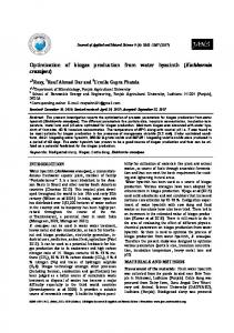
The energy production from biogas is based on renewable resources like agricultural products and organic waste. Since governmental funding for biogas plants will be reduced in the next years, biogas production has to be competitive to traditional energy sources such as nuclear power or fossil energy sources. The production of biogas is based on a broad variety of products, e.g., wheat or biological waste like animal manure. The biochemical process is realized by several species of bacteria in a multi-level process of anaerobic fermentation. The target of this process is to gain a maximum amount of methane (CH4 ). The result depends mainly on the amount and composition of the incoming substrate but as well on several different constraints like temperature, pH-value, and digester load. Due to the complexity of this process it is very difficult to predict the resulting amount of methane—especially when several substrates in different mixtures are used. We use a calibrated model to solve this task: The anaerobic digestion model no.1 (ADM1) (Batstone et al., 2002). The Matlab/Simulink toolbox Simba implements this model. Thus prediction of process results is a difficult task, but it is an unavoidable precondition to solve the more complex and sophisticated task of optimization. This optimization problem will be referred to as optimization of the biogas simulation in the following. The methane production is improved by optimizing the mixture of three substrates as input to the biochemical process. Constraints like minimal energy input or optimal digester load will also be considered. State of the art algorithms from computational intelligence (CI) are used to solve this optimization via simulation task. These algorithms were used with default parameter settings as well as with tuned parameters. Sequential parameter optimization (SPO) is used to tune the CI algorithms (Bartz-Beielstein et al., 2005). Figure 1 illustrates the situation. ∗ J¨ org Ziegenhirt, Thomas Bartz-Beielstein, Oliver Flasch, Wolfgang Konen, and Martin Zaefferer are with the Department of Computer Science and Engineering Science, Cologne University of Applied Science, 51643 Gummersbach, Germany (email: {joerg.ziegenhirt}@fh-koeln.de)

1

algorithm parameter set set of simulated organic waste mixtures simulated organic waste mixture

organic waste mixture

L4. L4.tuning tuningprocedure procedure

L3. optimization algorithm

L2. simulation model

optimized algorithm parameter optimized organic waste mixture

process parameters, estimated methan

methan

L1. L1.biogas biogasplant plant

input

output

Figure 1: Optimization via simulation. Four different layers of the biogas simulation. The first layer (L1) represents the real-world setting. Layer 2 (L2) shows the ADM1 simulator. The optimization algorithm, e.g., CMA-ES, belongs to the third layer (L3). The fourth layer (L4) represents the algorithm tuning procedure, e.g., sequential parameter optimization. The results will be compared to the results derived by Wolf et al. (2008). They applied genetic algorithms (GA) and particle swarm optimization (PSO) to solve the optimization of the biogas simulation task. This paper is organized as follows: A description of the biogas plant (L1), the related simulation model (L2), and the objective function (L3) is given in Sec. 2. Section 3 describes the goals of this study. The optimization algorithms (L3) are presented in Sec. 4. Section 5 describes the experiments and the tuning procedure (L4). Results are discussed in Sec. 6. Section 7 gives a summary and an outlook.

2 2.1

Optimization of the Biogas Plant Simulation The Biochemical Process

The simulation will be realized by a calibrated ADM1 model (Batstone et al., 2002; Wolf, 2005; Wolf et al., 2008). Though the ADM1 model did not change, its calibration was improved during the last years. To obtain comparability with the results from Wolf (2005), the simulations were repeated with the calibrated model before a comparison is done. The simulation of the biogas model is based on a period of 500 days to cover the whole startup period of the biogas plant. The plant is an agricultural plant configured to produce energy at a scale of 300 kWh. The energy production depends on the amount of methane generated during the biochemical process. Substrate quantity and quality have an significant impact on the methane production. In addition, the biochemical process is influenced by temperature or pH-value of the substrate. This adds further constraints

2

to the biogas simulation. The substrates in use are a mixture of agricultural products like wheat, corn-cob mix, or rye mash and organic waste like animal manure derived from chicken or pigs. The biochemical process that transforms this feed material into biogas is divided into several steps of an anaerobe fermentation process. Several different bacteria transform the material into methane and unwanted carbon dioxide (CO2 ). The simulation calculates the production of CH4 , CO2 , and hydrogen (H2 ) based on the mixture of the substrate. The simulation also calculates the amount of energy that will be obtained. The production of methane and its proportion in the resulting gas mixture has the largest effect on the energy output. The proportion of methane exceeds 50% in most cases, H2 usually less than 1%, whereas the remainder consists of CO2 . All other gases, which may be found in traces in the mixture, are not considered in the biogas simulation model. The exact proportions of the gas mixtures are one of the results of the simulation. The biogas simulator (from layer L2) provides additional information, which can be used to determine precise fitness function values. The steps of the biochemical process can be explained as follows. First step is the segmentation of the carbohydrate and protein of the substrates into their biological components. This step is called hydrolyse. It produces amino acids, fatty acids, and sugars—a process which is caused by enzymes which are produced by bacteria. The second step is called acidogenesis. Bacteria convert the biochemical substance derived from the first step into subsidiary fatty acid, CO2 , and water. Furthermore there are byproducts like alcohol and lactic acid. The third step is called acetogenese. Bacteria are now starting the production of acetic acid, hydrogen, and CO2 . The last step is usually considered as a part of the acetogenese. Bacteria are transforming the acetic acid in the final resulting gas methane and the byproduct CO2 .

2.2

Fitness Function

The optimization of the biogas simulation model (L2) may be seen as a black box optimization task. The input parameters and the relevant output parameters are chosen to estimate a valid model of the real-world biogas process from layer L1. The simulation part is slowing down the whole optimization process, because it is very time consuming. One run of the biogas simulation model ADM1 takes approximately ten seconds on a workstation. The input of the biogas plant is the substrate that is submitted, the output is mainly the energy that is produced. To define a fitness function, we have to divert the problem into more specific values: The mixture of the input consists of three different substrates inserted to the biogas plant: 1. rye (Rye), 2. corn-cob mix (CCM ), 3. and pigs manure (M an). The ADM1 simulator is started with these inputs and the results obtained lead to multiple result information. The fitness function has to consider several different targets, so we have a multi criteria fitness function that combines eight different targets: 1. the fermentation progress (Ds ), 2. the energy consumption for digester heating (Eh ), 3. the quality of the gas produced (Gq ), 4. the amount of methane produced (Ga ), 5. the contamination of the digestion tank (Ld ), 6. a penalty term for exceeding the limit for the pH-value (PpH ), 7. a penalty term for exceeding the limits given for the substrate input (Ps ), 8. and the share of dry substrate (PT S ). 3

Each target is normalized to a value between zero and one. The limits are derived by the limitations of the real-world plants from layer L1 or are given by the carrier. The main target, i.e., the production of the methane, should not exceed a certain limit due to economical reasons: if the amount of 2,200 m3 gas is exceeded, the revenue guaranteed will be reduced. As a result we obtain the following fitness function: f =c1 · Ds + c2 · Eh + c3 · Gq + c4 · Ga + c5 · Ld + c6 · PpH + c7 · Ps + c8 · PT S

(1)

The factors c1 −c8 are used as weights for each term of the fitness function. The variables Ga and Ld are the most important targets. The best algorithm to scale the weights would be their economical share but there is no mathematical equation to calculate their influence objectively. Consequently, recommendations from plant operators are used for calibrating the weights. We formulate the optimization task as a minimization problem.

3

Research Goals

Fast and reliable simulation models are of great importance for the practitioner. The study of Wolf et al. (2008) was used as a starting point for our research. Based on demands from biogas simulation practice in real-world scenarios, we formulate the following goals: G-1 Determine a CI algorithm that improves the optimization of the biogas simulation significantly, i.e., the optimization is more effective and efficient (Bartz-Beielstein, 2006). G-2 Realizing a very significant execution time decrease without any loss of solution quality by tuning a CI algorithm found by G-1.

4

CI algorithms

The algorithms from optimization layer (L3) are presented in this section.

4.1

Genetic Algorithm

The GA examined in this comparison is based on the implementation of the genetic algorithm and direct search (GADS) toolbox from Matlab. The algorithm is started with exactly the same parameters that were used by Wolf et al. (2008). They are shown in Table 1.

4.2

Particle Swarm Optimization

PSO was the second CI algorithm investigated by Wolf et al. (2008). The PSO is an implementation available as free toolbox for Matlab (Birge, 2006). The best parameters found and discussed before are listed in Table 1.

4.3

CMA-Evolution Strategy

The Matlab implementation of the covariance matrix adaptation evolution strategy (CMA-ES) from Hansen (2009) was used in our experiments. The default parameters for the CMA-ES are defined as shown in Table 2.

4.4

Differential Evolution

Finally, we added differential evolution (DE) to our CI algorithm portfolio (Price et al., 2005). Here, the Matlab implementation available from Price and Storn (2010) was chosen. The parameter settings used to start the optimization lead to a setting that is used for small population size and fast convergence. According

4

Table 1: GA and PSO Parameter Settings GA parameter value number of generations 200 population size 60 probability of crossover 0.7 crossover strategy intermediate mutation strategy adaptive feasible selection strategy elitism + stochastic uniform PSO parameter value number of particles 30 number of iterations 400 personal best influence 2 global best influence 2 initial inertia weight 0.9 final inertia weight 0.6

Table 2: CMA-ES and DE Parameter Settings CMA-ES parameter value sigma0 3 popsize 30 DE parameter value strategy DE/best/1 with jitter population size 30 crossover rate 1 step-size weight 0.8

5

to recommendations for this scenario, population size should be ten times the dimension of the problem. Crossover rate and step-size weight were set to their default values, see Table 2. Whereas GA and PSO were chosen to enable a comparison with existing results, the CMA-ES and DE were chosen because of their good performance in the CEC 2005 comparison of evolutionary algorithms on a benchmark function set (Hansen, 2005). The CMA-ES was chosen as state of the art algorithm and best in the benchmark. To have a qualifying comparison the second of the benchmark tests in Hansen (2005), i.e., DE, is included in our comparison.

5

Experiments: Setup and Results

5.1

Considering Parameter Settings

Parameter settings can influence the performance of algorithms significantly. To avoid misinterpretation of results from comparisons caused by wrongly parametrized algorithms, we compare results from runs with • default parameter settings and • improved (tuned) parameter settings. Note, these parameter settings refer to layer L3 from Fig. 1. SPO was used to tune these parameters. It is a flexible and general framework which can be applied in many situations. The related toolbox (SPOT) was developed over recent years by Thomas Bartz-Beielstein, Christian Lasarczyk, and Mike Preuss (BartzBeielstein et al., 2005). The main purpose of SPOT is to determine improved parameter settings for optimization algorithms to analyze and understand their performance. SPOT was successfully applied to numerous optimization algorithms, especially in the field of evolutionary computation, e.g., evolution strategies, particle swarm optimization or genetic programming. It was applied in various domains, e.g., machine engineering, the aerospace industry, bioinformatics, CI and games as well as in fundamental research (Beume et al., 2008; Henrich et al., 2008; Lucas and Roosen, 2009; Preuss et al., 2007; Fialho et al., 2009; Fober et al., 2009; Stoean et al., 2009; Hutter et al., 2010). During the first stage of experimentation, SPOT treats the algorithm A from layer L3 as a black box. A set of input variables, say ~x, is passed to A. Each run of the algorithm produces some output, ~y . SPOT tries to determine a functional relationship F between ~x and ~y for a given problem formulated by an fitness function f : ~u → ~v . Note, the fitness function values are generated in layer L2. This situation can be described as follows: L2: Fitness function: L3: Algorithm:

f

~u −→ ~v , F

~x −→ ~y ,

(2) (3)

where ~x is the set of (simulated) substrate mixtures, ~y the best substrate mixture found in a certain run of the optimization algorithms from layer L3, ~u the (simulated) substrate mixture, and ~v results generated by one run of the ADM1 biogas simulator (L2) which is used in Eq. 1 to determine the fitness value f . We will classify elements from Eq. 2 and Eq. 3 in the following manner: 1. Variables that are necessary for the algorithm (from layer L3) belong to the algorithm design, whereas 2. variables that are needed to specify the optimization problem f (from layer L2) belong to the problem design. Residing on layer L4, SPO employs a sequentially improved model to estimate the relationship between values from the algorithm design and the corresponding output. This serves two primary goals. One is to enable determining good parameter settings, thus SPOT may be used as a tuner. Secondly, variable interactions can be revealed that help to understand how the tested algorithm works when confronted with a specific problem or how changes in the problem influence the algorithm’s performance. Concerning the model, SPOT allows for insertion of virtually every available model. However, regression and Kriging models or a combination thereof are most frequently used. Here, we employ a recently developed Kriging approach which is able to cope with stochastically disturbed input values (Bartz-Beielstein, 2010). 6

2 GA PSO

1.98 1.96

Fitness

1.94 1.92 1.9 1.88 1.86 1.84 1.82 1.8

0

2000

4000 6000 8000 Function evaluations

10000

12000

Figure 2: Fitness (see Eq. 1) plotted versus number of function evaluations. Results from the GA and PSO runs which are taken as reference algorithms in our study. PSO and GA required 12,000 function evaluations. 2.2 GA PSO DE CMA−ES

2.15 2.1

Fitness

2.05 2 1.95 1.9 1.85 1.8

0

500

1000 1500 Function evaluations

2000

Figure 3: Fitness (see Eq. 1) plotted versus number of function evaluations. Results from experiment E-1. Same setting as in Fig. 2, but only 2,000 function evaluations. DE and CMA-ES included in the set.

5.2

Comparable Simulation Results

Results from Wolf (2005) and Wolf et al. (2008) are not directly comparable to results from our study, because the calibration of the ADM1 biogas simulation model used for the evaluation changed in the meantime. These modifications were caused by adaptations of the ADM1 model (layer L2) to real behavior (layer L1) and led to an improvement of the calibrations from Wolf (2005) and Wolf et al. (2008). Therefore the simulation runs were repeated with the new calibrations to generate comparable simulation results and fitness values. The fitness function evaluation, which is performed in layer L2, is the same for all algorithms in this comparison. Each configuration is evaluated 10 times with different seeds to avoid interpretations that were disturbed by noise. 10 is a small figure, but the evaluation time is about 10 seconds for each evaluation on an actual workstation, so it is considered a good compromise with statistically soundness and manageable in a reasonable time. All conclusions made in this research are based on a repetition of the settings with 10 different seeds usually presented as a mean value as long as the standard deviation is not significant. The validation of the results had to be done with 12,000 fitness evaluations, i.e., ADM1 simulator runs. The results depicted in Fig. 2 show a faster convergence of the GA. However, after 2,000 function evaluations, GA is outperformed by PSO. The 10 repeats of the GA 7

1.88

1.87

1.86

1.85

1.84

1.83

1

2

3

4

Figure 4: Experiment E-1: Boxplots comparing the performance of PSO (1), GA (2), CMA-ES (3), and DE (4). Each algorithm was run ten times with different random seeds. Smaller values are better. Note, data from CMA-ES (3) and DE (4) are also shown in Fig. 6 reach a mean value of 1.86 for this minimization task, whereas PSO finds a value of 1.83. Taking 12,000 function evaluations into account, Wolf et al. (2008) concluded that PSO performs better than GA.

5.3

Searching for Improved Algorithms

Now that comparable results for PSO and GA are available, we start runs with state-of-the-art CI algorithms. This leads to the following experiment. E-1: Comparison of CMA-ES and DE with default parameter settings to GA and PSO with parameter settings used by Wolf et al. (2008). Results from this experiment are shown in Fig. 3. The fitness values delivered from CMA-ES and DE show initially a faster convergence than PSO. Even more, they lead after 1,200 evaluations to fitness values considerably better than both GA and PSO. The value reached by CMA-ES after 1,200 evaluations remains constant throughout the next 10,000 evaluations. Therefore, CMA-ES and DE required one tenth of the simulation time used by GA and PSO. They obtained even better results than GA or PSO with a reduced number of function evaluations as can be seen in Fig. 4. In order to define a good compromise between robustness of the results and manageability in time a number of 2,000 function evaluations was considered to be sufficient for the biogas simulation runs. Since goals G-1 and G-2 have been reached at this stage of experimentation, we decided to perform further experiments which might lead to additional improvements.

5.4

Tuning DE and CMA-ES with SPOT

SPOT provides methods to determine improved parameters for algorithms such as DE and CMA-ES. For this examination the number of calls of each set of parameters was decreased to tmax =1,000 fitness evaluations only. To reduce the time for these evaluations, the simulation model was called with a reduced number of days (50 days). Note, that this is just an approximation to the final ADM1 simulation and hence optimization algorithm value. The best parameters found for an optimization algorithm is used to run the algorithm ten times with a full simulation period of 500 days. The second experiment from our study can be formulated as follows: E-2 Determine an improved parameter setting for DE. DE has a set of six strategies implemented in Matlab. These should be treated as categorical values, say A, B, C, . . . F . One possible, but inefficient way for numerical optimization algorithms to cope with

8

Table 3: DE Parameter Settings for SPOT DE Parameter Region of Interest Best found popsize 5..50 29 crossover ratio 0.0..1.0 0.83 step-size weight 0.0..2.0 0.55

Table 4: CMA-ES Parameter Settings for SPOT CMA-ES Parameter Region of Interest Best found nparents 1..10 4 popsize 2..100 12 tccs 0.0..0.9 0.24 damps 0.0..5.0 1.58

categorical variables is to treat these variables as numerical variables. Alternatively, separate runs for each level of the categorical variable can be performed, which is also computationally expensive. SPOT offers an efficient way to handle this problem, because it provides several optimization tools which can be applied to numerical and nonnumerical variables. We performed a two-stage SPOT approach here. 1. During the first stage, categorical variables are included in SPOT’s region of interest (search space). To cope with nonnumerical values, a tree-based approach was chosen for building SPOT’s prediction model. 2. The second stage uses the best setting of the categorical variable which was determined in the first phase, e.g., strategy C. Here, numerical parameters are optimized by SPOT. In our experiments, a first SPOT run was performed in order to determine the best DE strategy. The strategy “DE/best/1 with jitter” was identified. Note, this was the same strategy which was used already in the first comparison, i.e., experiment E-1. Then this strategy was investigated to find the best parameters for by SPOT. Therefore SPOT was started 60 times with a complete DE run. As a sum we had 60,000 evaluations to find better parameter settings for the DE. The parameters identified that could be adapted are shown in Table 3. The results will be shown together with the next experiment in Fig. 5. E-3: Determine improved parameter settings for the CMA-ES. In contrast to DE, CMA-ES does not require a two-stage approach, because it does not use categorical variables. So CMA-ES can be optimized by SPOT right away. The runs were also started 60 times which gives a total number of 60,000 evaluations to determine the parameter settings. Figure 5 illustrates results from CMA-ES and DE with default and tuned parameters. Since these algorithms reach nearly optimal values after tmax = 1, 000 function evaluations, we reduced tmax to 1,000. Note, results for algorithms with default parameter settings for tmax = 2, 000 were shown in Fig. 3. Obviously, the SPOT tuned algorithms did not find better results than algorithms with default parameter settings. Boxplots which illustrate results from ten runs of each algorithm are shown in Fig. 6. However, results from experiments E-2 and E-3 indicate that SPOT was able to improve the efficiency of the algorithms, i.e., they converge faster to the (local) optimum. This observation motivated an additional experiment, which will be described in the following section.

5.5

SPOT and CMA-ES Hybridization

It might be interesting to see if SPOT is able to improve the efficiency of the optimization algorithms. Efficiency is related to the question: Does the algorithm produce the desired effects without waste (BartzBeielstein, 2006)? Superfluous function evaluations are considered as waste in this context. 9

2.1 DE CMA−ES CMA−ES SPOT DE SPOT

2.05

Fitness

2 1.95 1.9 1.85 1.8

0

200

400 600 Function evaluations

800

1000

Figure 5: Results from experiments E-2 and E-3. Comparison default to SPOT tuned DE and CMA-ES

1.8321

1.832

1.832

1.8319

1

2

3

4

Figure 6: Comparison of CMA-ES (1) and DE (2) with default parameter settings, CMA-ES (3) and DE (4) with tuned parameters. Note, boxplots CMA-ES (1) and DE (2) are based on the same data as CMA-ES (3) and DE (4) in Fig. 4. Differences became visible due to a different scaling

10

2.2 CMA−ES SPOT 200 CMA−ES SPOT 1000 CMA−ES DE

2.15 2.1

Fitness

2.05 2 1.95 1.9 1.85 1.8

0

50

100 150 Function evaluations

200

Figure 7: Fitness (see Eq. 1) plotted versus number of function evaluations. Results from the different SPOT tuned CMA-ES versus untuned CMA-ES and DE for the first 200 evaluations Table 5: Experimental setup for E-1 to E-4

spot budget spot tmax tmax repeats

E-1 GA PSO 12000 10

E-1 DE CMAES 2000 10

E-2

E-3

E-4

DE 50 1000 2000 10

CMAES 50 1000 2000 10

CMAES 5 200 1000 10

To enable a fair comparison, a total number of 2,000 function evaluations, i.e., simulator runs from layer L2, are allowed in this experiment, which can be specified as follows: E-4 Use 50% of the available function evaluations for algorithm tuning and perform the algorithm run with the other half. The budget of 2, 000 function evaluations was split into 1,000 evaluations assigned to SPOT and 1,000 for a final CMA-ES run. SPOT uses five runs of the algorithm (layer L3) to estimate the algorithm’s performance. Each run requires 200 simulator runs (from layer L2), which results in 5 × 200 = 1, 000 runs of the simulation model. Based on these five runs a meta-model is generated. The meta-model is used to determine an improved algorithm parameter setting (CMA-ES200), which is used for one long algorithm run (1,000 runs of the simulator). Altogether 5 × 200 + 1, 000 = 2, 000 simulator runs are required. This method can be considered as a hybrid approach, because two optimization strategies are combined. Figure 7 compares results from the CMA-ES200 with results from the other algorithms of this study. It can be seen that CMA-ES200 performs better than the default CMA-ES. Its performance is comparable to the CMA-ES1000 (where 1,000 evaluations were allowed during the tuning process, see Sec. 5.4). However, if CMA-ES200 is run for 1,000 function evaluations, the situation changes: the other algorithms perform significantly better than the CMA-ES200. One possible explanation for this behavior may be the fact that CMA-ES was tuned for 200 function evaluations. Figure 8 illustrates these results. Table 5 summarizes the experimental setup for E-1 to E-4: spot budget denotes the number of algorithm runs from L3, which is used during the SPOT tuning process; spot tmax is the number of fitness function evaluations from L2 used by the algorithm during the SPOT tuning process, tmax is the number of fitness function evaluations from L2 used during the optimization runs, and repeats denotes the number of repeats used in the comparison. Note, a two-stage approach was used for E-2. For the first stage, which was performed as a SPOT tuning of the categorical variables, a budget of 25 algorithm runs from layer L3 with tmax = 1000 fitness function evaluations from layer L2 were chosen.

11

2 CMA−ES SPOT 200 CMA−ES SPOT 1000 CMA−ES DE

1.98 1.96

Fitness

1.94 1.92 1.9 1.88 1.86 1.84 1.82 1.8

200

400 600 Function evaluations

800

1000

Figure 8: Fitness (see Eq. 1) plotted versus number of function evaluations. Same setting as in Fig. 7, but focused on the progress made in the last 900 evaluations of the run. Table 6: Pairwise comparisons using t tests with non-pooled SD, p value adjustment method: Holm. CMAES+ and DE+ denote the SPOT tuned versions of CMA-ES and DE, respectively CMAES+ DE DE+ GA PSO

5.6

CMAES 1.00000 1.00000 0.24582 0.00010 0.01716

CMAES+ 1.00000 1.00000 0.00010 0.01716

DE 0.52958 0.00010 0.01716

DE+ 0.00010 0.01716

GA 0.50775

Multiple Comparisons

In addition to the graphical comparisons shown in Figs. 4 and 6, we performed a statistical analysis of the data from experiments E1-E-4, see Table6. We calculated pairwise comparisons between group levels with corrections for multiple testing (Holm, 1979). The tests were performed without using a common pooled standard deviation, because we do not assume equal variance for all groups, i.e., algorithms. Results from this analysis are in accordance with conclusions drawn from the boxplots: For example, GA performs worse than CMA-ES (p value 0.0001), and PSO and GA show no statistically significant difference in their performances (p value 0.50775).

6

Discussion

Results from experiment E-1 clearly demonstrate that CMA-ES and DE were able to obtain optimal results significantly faster than PSO and GA. Thus, goals G-1 and G-2 were reached. This result is a valuable indicator that results from the CEC 2005 test suite (Hansen, 2005) can be transferred to real-world settings. Experiments E-2 and E-3 indicate, that no significant further improvement can be obtained for this setting, even if parameter tuning methods are used. DE and CMA-ES were able to reach the basin of attraction of the optimization of the biogas simulation problem with their default parameterizations. Furthermore, we assume that the instance of the biogas simulation problem considered in this study has a local minimum (with a fitness function value close to 1.8). This implies that there is not much space for improvement which can be exploited by the tuning algorithm, e.g., SPOT. The analysis of one algorithm run may give some further insight. Figure 9 illustrates the proportion of the substances which are the input to the simulation model from layer L2. Only marginal improvements can be observed after 500 function evaluations—the proportions remain constant. A contour plot of the fitness landscape supports this assumption, see Fig. 10. There is a large diagonal basin of attraction.

12

Object Variables (3−D) 10 Rye=8.66 8 Man=6.97

m³

6

4 CCM=1.51

2

0

0

500

1000 1500 Function evaluations

2000

Figure 9: Development of the best individual throughout one complete run. The proportion of substances of the mixture during a run of CMA-ES is illustrated. The amount in m3 of pig manure (Man), corn-cob mix (CCM), and rye (Rye) is plotted for the best individual found at each evaluation step.

f 0

m

5

10 16

m 15

14 10 12

5

ccm

10

0

m

m

8

15 6 10 4

5 2

0

0 0

5

10

r

Figure 10: Contour plot of the fitness function f as defined in Eq. 1. Values are based on results from one CMA-ES run. Corn-cob mix (ccm) is plotted versus rye (r), while values of pigs manure (m) are varied with the slider on top of each panel. Optimal fitness function values are located along the main diagonal. Contour lines are nearly parallel

13

Results from experiment E-4 indicate that the parameter tuning process depends on the prespecified number of function evaluations, i.e., the computational budget tmax . An algorithm tuned for, say tmax = 200, might perform worse if tmax is increased (or decreased). This observation needs further investigations, because it is based on one optimization (via simulation) problem only.

7

Summary and Outlook

The results of the optimization runs with different algorithms showed that both, CMA-ES and DE, might be very well applicable to the problem of biogas plant optimization. Both algorithms largely outperform the reference algorithms GA and PSO. Further investigations on real world driven constraints can be included easily to reach fast responses to a changing environment. Further improvements in quality and speed by tuning the algorithms with SPOT could not be observed to a significant extent. Nevertheless the SPOT tuned algorithms show a significant correlation to the number of fitness function they were tuned with. A behavior that should be subject to further investigation. Answering requests from biogas industry, we will consider extensions of the fitness function (Eq. 1), e.g., by including additional substrates. Effects of theses extensions on the performance of the CMA-ES and DE are subject of further research.

Acknowledgments This work has been supported by the Bundesministerium f¨ur Forschung und Bildung (BMBF) under the grants FIWA (AIF FKZ 17N2309, ”Ingenieurnachwuchs”) and by the Cologne University of Applied Sciences under the research focus grant COSA. We are grateful to Prof. Dr. Michael Bongards and his research group (GECO-C) for discussions and for the biogas plant data and software and to Christian Wolf for making results from his ADM1 simulations available to us as well as for many helpful discussions.

References D. J. Batstone, J. Keller, I. Angelidaki, S. V. Kalyuzhnyi, S. G. Pavlostathis, A. Rozzi, W. Sanders, H. Siegrist, and V. A. Vavilin, “Anaerobic Digestion Model No. 1, Scientific and technical report no.13,” IWA Task Group for Mathematic Modelling of Anaerobic Digestion Processes, London, Tech. Rep., 2002. T. Bartz-Beielstein, C. Lasarczyk, and M. Preuß, “Sequential parameter optimization,” in Proceedings 2005 Congress on Evolutionary Computation (CEC’05), Edinburgh, Scotland, B. McKay et al., Eds., vol. 1. Piscataway NJ: IEEE Press, 2005, pp. 773–780. C. Wolf, S. McLoone, and M. Bongards, “Biogas plant optimization using Genetic Algorithms and Particle Swarm Optimization,” Signals and Systems Conference, ISSC, vol. 208, pp. 244–249, 2008. ¨ C. Wolf, “Entwicklung und experimentelle Uberpr¨ ufung eines Simulationsmodells zur Regelungstechnischen Optimierung landwirtschaftlicher Biogasanlagen,” Diplomarbeit, Fakult¨at f¨ur Informatik und Ingenieurwesen, Fachhochschule K¨oln, Germany, 2005. T. Bartz-Beielstein, Experimental Research in Evolutionary Computation—The New Experimentalism, ser. Natural Computing Series. Berlin, Heidelberg, New York: Springer, 2006. B. Birge, “Particle Swarm Optimization toolbox,” Matlab: www.mathworks.com/matlabcentral, 2006. N. Hansen, “CMA evolution strategy source code,” www.lri.fr/∼hansen/cmaes inmatlab.html, 2009.

14

K. V. Price, R. M. Storn, and J. A. Lampinen, Differential Evolution: A Practical Approach to Global Optimization. Berlin, Germany: Springer, 2005. K. V. Price and R. M. Storn, “Differential Evolution (DE) for Continuous Function Optimization,” www. icsi.berkeley.edu/∼storn/code.html, 2010. N. Hansen, “Comparison of Evolutionary Algorithms on a Benchmark Function Set,” www.lri.fr/∼hansen/ cec2005.html, 2005. N. Beume, T. Hein, B. Naujoks, N. Piatkowski, M. Preuss, and S. Wessing, “Intelligent Anti-Grouping in Real-Time Strategy Games,” in IEEE Symposium on Computational Intelligence and Games (CIG 2008). Piscataway, NJ: IEEE Press, 2008. F. Henrich, C. Bouvy, C. Kausch, K. Lucas, M. Preuß, G. Rudolph, and P. Roosen, “Economic optimization of non-sharp separation sequences by means of evolutionary algorithms,” Computers and Chemical Engineering, vol. 32, no. 7, pp. 1411–1432, 2008. K. Lucas and P. Roosen, Emergence, Analysis and Optimization of Structures: Concepts and Strategies Across Disciplines. Springer Verlag, 2009. M. Preuss, G. Rudolph, and F. Tumakaka, “Solving multimodal problems via multiobjective techniques with Application to phase equilibrium detection,” in Proceedings of the International Congress on Evolutionary Computation (CEC2007). Piscataway (NJ): IEEE Press. Im Druck. Citeseer, 2007. ´ Fialho, M. Schoenauer, and M. Sebag, “Analysis of adaptive operator selection techniques on the royal A. road and long k-path problems,” in Proceedings of the 11th Annual conference on Genetic and evolutionary computation. ACM, 2009, pp. 779–786. T. Fober, M. Mernberger, G. Klebe, and E. Hullermeier, “Evolutionary construction of multiple graph alignments for the structural analysis of biomolecules,” Bioinformatics, vol. 25, no. 16, p. 2110, 2009. C. Stoean, M. Preuss, T. Bartz-Beielstein, and R. Stoean, “A new clustering-based evolutionary algorithm for real-valued multimodal optimization,” Chair of Algorithm Engineering, TU Dortmund, Dortmund, Germany, Tech. Rep. TR09-2-007, 2009. F. Hutter, T. Bartz-Beielstein, H. Hoos, K. Leyton-Brown, and K. P. Murphy, “Sequential model-based parameter optimisation: an experimental investigation of automated and interactive approaches empirical methods for the analysis of optimization algorithms,” in Empirical Methods for the Analysis of Optimization Algorithms, T. Bartz-Beielstein, M. Chiarandini, L. Paquete, and M. Preuss, Eds. Berlin, Heidelberg, New York: Springer, 2010, pp. 361–414. T. Bartz-Beielstein, “Kriging based sequential parameter optimization,” submitted for publication, 2010. S. Holm, “A simple sequentially rejective multiple test procedure,” Scandinavian Journal of Statistics, vol. 6, pp. 65–70, 1979.

15