Optimization of bodies with locally periodic microstructure

Optimization of bodies with locally periodic microstructure Cristian Barbarosie Anca-Maria Toader Preprint CMAF Pre-2009-021 http://cmaf.ptmat.fc.ul.pt/preprints.html {barbaros,amtan}@ptmat.fc.ul.pt December 2, 2009

Abstract This paper describes a numerical study of the optimization of elastic bodies featuring a locally periodic microscopic pattern. Our approach makes the link between the microscopic level and the macroscopic one. Two-dimensional linearly elastic bodies are considered; the same techniques can be applied to threedimensional bodies. Homogenization theory is used to describe the macroscopic (effective) elastic properties of the body. The macroscopic domain is divided in (rectangular) finite elements and in each of them the microstructure is supposed to be periodic; the periodic pattern is allowed to vary from element to element. Each periodic microstructure is discretized using a finite element mesh on the periodicity cell, by identifying the opposite sides of the cell in order to handle the periodicity conditions in the cellular problem. Shape optimization and topology optimization are used at the microscopic level, following an alternate directions algorithm. Numerical examples are presented, in which a cantilever is optimized for different load cases, one of them being multi-load. The problem is numerically heavy, since the optimization of the macroscopic problem is performed by optimizing in simultaneous hundreds or even thousands of periodic structures, each one using its own finite element mesh on the periodicity cell. Parallel computation is used in order to alleviate the computational burden.

Key-words shape optimization, topology optimization, alternate directions algorithm, locally periodic homogenization, cellular problem, parallel computation 1

1

Introduction

The main motivation of the present paper comes from the study of bodies having locally periodic microstructure and optimization of their macroscopic properties, in the context of linearized elasticity. A body having locally periodic microstructure is a body whose material coefficients vary at a microscopic scale, and this variation is locally periodic in the sense that, around each point of the body, the material coefficients vary according to a periodic pattern. This pattern changes from point to point (at the macroscopic scale). Homogenization theory allows one to accurately describe the macroscopic behaviour of such a body by means of so-called cellular problems, which are elliptic PDEs subject to periodicity conditions, see e.g. [1], [2]. Porous materials, that is, bodies with locally periodic infinitesimal perforations, can be described in a similar manner, see [3]. In [4] and [5], the authors have presented results for the optimization of periodic structures. The present paper represents a natural continuation, linking the microscopic level to the macroscopic problem. Preliminary results were presented in [6]. The layout of the paper is as follows. Section 2 introduces the notion of periodic microstructure and the associated homogenized elastic tensor. Section 3 describes locally periodic microstructures. Section 4 presents the shape and topology derivatives, that is, the sensitivity of the objective functional to infinitesimal variations in the shape or topology of the microscopic holes. Section 5 describes the optimization algorithm, together with some implementation details. Section 6 presents several examples of optimization of locally periodic structures. Note that a similar approach was proposed in [7] with a different treatment of the cellular problem.

2

Periodic microstructures

As a preliminary for describing mathematically the notion of body having locally periodic microsctructure, we shall introduce the notion of periodic microstructure. We shall use notations and results from [4]. Consider a parallelepiped Y in Rn (a parallelogram in R2 ) which defines the periodicity of the microstructure. Often Y is taken to be the unit cube for the sake of simplicity. A periodic microstructure is a body whose material coefficients (i.e., for the case of linear elasticity, its rigidity tensor) varies according to a periodic pattern C, which is a Y -periodic fourth-order tensor field C : Rn → Rn×n×n×n . Typically, but not necessarily, the pattern tensor field C takes only two values, modeling a periodic mixture between two given component materials (see Figure 1). The effective (macroscopic) behaviour of the body is described by the socalled homogenized elastic tensor, denoted by CH and defined in terms of solu-

2

Figure 1: Periodic mixture of two materials tions of elliptic partial differential equations subject to periodicity conditions. More precisely, for a given macroscopic strain (represented by a symmetric n×n matrix A), consider the problem  −div(C ǫ(wA )) = 0 in Rn (1) wA (y) = Ay + φA (y), with φA Y −periodic, known in homogenization theory as cellular problem. Here, ǫ represents the symmetric part of the gradient. The solution wA of the above problem depends (linearly) on the matrix A. Consequently, the matrix σ defined by Z 1 σ= C ǫ(wA ) , |Y | Y representing the macroscopic stress associated to wA , depends linearly on the macroscopic strain A and this dependency defines the homogenized elastic tensor CH through CH A = σ, that is, Z 1 H C ǫ(wA ) . C A= |Y | Y In the above, |Y | denotes the volume of the periodicity cell Y (its area, in two dimensions). An equivalent definition of CH can be given in terms of energy type products : for two given symmetric matrices A and B, one has Z 1 H hC A, Bi = hC ǫ(wA ), ǫ(wB )i . |Y | Y Note that, for a function wA of the form wA (y) = Ay+φA (y), with φA Y -periodic, one has Z 1 A= ǫ(wA ) , |Y | Y see in [4] Lemma 1 and its consequences. This can be expressed in a more concise form by introducing the set of linear plus periodic functions denoted by LP = {w : Rn 7→ Rn | w(y) = Ay + ϕ(y) , A ∈ Mn (R), 1 ϕ ∈ Hloc (Rn ; Rn ) and Y − periodic}, 3

Y T

Figure 2: Periodicity cell with model hole (zoomed)

Figure 3: Periodically perforated plane R2perf The cellular problem (1) may be written in strain formulation as follows:  wA ∈ LP  −div(CRǫ(wA )) = 0 in Rn  1 |Y | Y ǫ(wA ) = A ,

(2)

where A ∈ Mn (R) is a given strain matrix. The case of porous structures, that is, infinitesimal perforations in a given material, can be treated in a similar way, see [4], Section 4. Consider a model hole, which is a compact set T ⊂ Y (see Figure 2), where Y is the periodicity cell. The cellular problem describing the behaviour of this perforated material is defined on the perforated space, denoted by Rnperf , and a Neumann boundary condition is imposed on the boundary of the model hole. The perforated space is obtained from Rn by removing translations of the model hole (see Figures 3 and 4). For an arbitrary parallelipiped Y defined by n linearly independent vectors ~g1 , ~g2 , . . . , ~gn , one has [ Rnperf = Rn \ (T + k1~g1 + k2~g2 + . . . + kn~gn ) ~ k∈Zn

The direct generalization of the cellular problem (1) for porous materials is

4

Figure 4: Periodically perforated plane R2perf for another cell stated below (the base material C is now considered to be constant) :  −div(C ǫ(wA )) = 0 in Rnperf  C ǫ(wA ) n = 0 on ∂T  wA (y) = Ay + φA (y), φA periodic function.

(3)

The homogenized tensor CH can be defined as Z 1 H C A= C ǫ(wA ) |Y | Y \T

or

1 hC A, Bi = |Y | H

Z

hC ǫ(wA ), ǫ(wB )i .

Y \T

Remark 1 Note that, through careful interpretetation, problems (3) makes sense even if the model hole T exits partially the periodicity cell Y , as long as it does not touch any of its translations T + ~k, ~k ∈ Zn , ~k 6= ~0. This is important since, in the optimization process, the model hole often crosses the boundary of Y . Remark 2 In the above, the model hole T was chosen to be connected. But there is no difficulty in considering a model hole with several connected components.

3

Locally periodic microstructures

We call “locally periodic” a microsctructure which, in the neighbourhood of each point of the macroscopic domain, has a periodic character. This periodic microgeometry can vary from point to point (at the macroscopic level). This corresponds to a pattern tensor field C depending on both x (the macroscopic variable) and y (the microscopic variable). The cellular problem (1) depends now on x as a parameter :
 −divy C(x, y) ǫy (wA (x, y)) = 0 in Rn (4) wA (x, y) = Ay + φA (x, y), with φA (x, ·) Y −periodic, 5

The homogenized elastic tensor CH depends now on x and is defined by Z 1 hCH (x)A, Bi = hC(x, y)ǫy (wA (x, y)), ǫy (wB (x, y))i dy , |Y | Y where A and B are two arbitrary strain matrices. A locally periodic porous material is described in a similar manner. The model hole T now varies with x and shall be denoted by T (x). The corresponding perforated space will be denoted by Rnperf (x) Rnperf (x) = Rn \

[

(T (x) + k1~g1 + k2~g2 + . . . + kn~gn )

~ k∈Zn

The base material C is now considered to be constant. The cellular problem (3) becomes
 −divy C ǫy (wA (x, y)) = 0 in Rnperf (x)  (5) C ǫy (wA (x, y))n = 0 on ∂T (x)  wA (x, y) = Ay + φA (x, y), φA periodic in y. The homogenized ellastic tensor CH (x) is defined by Z 1 hC ǫy (wA (x, y)), ǫy (wB (x, y))i dy , hCH (x)A, Bi = |Y | Y \T (x)

(6)

where A and B are two arbitrary strain matrices. Remark 3 In the present paper, we assume that the periodicity cell (which is the parallelipiped defined by n linearly independent vectors ~g1 , ~g2 , . . . , ~gn ) is constant in the macroscopic domain, in the sense that it does not vary with x. We may study examples involving different periodicity cells, but within each example, the cell will be constant. Letting the vectors ~g1 , ~g2 , . . . , ~gn depend on x, and also letting them vary during the optimization process, is the object of on-going work. The behaviour of the macroscopic body is described by the homogenized elastic tensor CH (x). More precisely, suppose that the macroscopic body occupies the domain Ω ⊂ Rn , that the boundary of Ω is split in two parts (the Neumann part ΓN and the Dirichlet part ΓD ) and that the body is subject to the superficial force g. Then, the state of the body u is the solution of  Ω  −divx (CH ǫx (u)) = 0 in (7) u=0 on ΓD  (CH ǫx (u))n = g on ΓN .

6

4

Shape and topology derivatives

The aim of the present paper is to optimize macroscopic properties of the body under study, by varying the details of its locally periodic microstructure, more specifically, by varying the shape and topology of the holes T (x). Consider an objective functional Φ depending on the solution u of problem (7). A typical example is the minimization of the compliance of the body Z Z Z gu − hCH ǫx (u), ǫx (u)i (8) gu = 2 Φ= Ω

ΓN

ΓN

Usually, there is also a constraint on the volume of material: Z θ, V =

(9)

Ω

where θ(x) =

|T (x)| |Y \ T (x)| =1− |Y | |Y |

is the local material density. So, one has to deal with a chain of dependencies : T 7→ CH 7→ u 7→ Φ , that is, to a family of cellular holes T (x) one associates the homogenized tensor CH (x) as defined by (6), then the macroscopic elastic deformation u as defined by (7) and finally the value of the objective functional Φ. A similar chain of dependencies exists for the volume V . For optimizing the properties of the considered structure, a gradient-based algorithm can be used. This is why infinitesimal variations in the shape and/or topology of the family of holes T should be considered and the corresponding variations in the chain of dependencies should be described : δT 7→ δCH 7→ δu 7→ δΦ .

(10)

Describing the variation δΦ of the objective functional in terms of δCH and δu is relatively simple. For the particular case here studied, see (8), one has Z Z Z g δu − hδCH ǫx (u), ǫx (u)i − 2 hCH ǫx (u), ǫx (δu)i δΦ = 2 Ω

ΓN

Ω

Remark 4 Eliminating δu from the formula of δΦ is usually a complicated task; this is done by expressing δu in terms of δCH and by making use of the adjoint equation. However, for the particular case of the compliance (8) this is not necessary, since the minimization of the compliance is a self-adjoint problem. For the case under study, it suffices to note that Z Z g δu = hCH ǫx (u), ǫx (δu)i . ΓN

Ω

7

Y T(x)

Figure 5: Infinitesimal deformation of the model hole T (x) The above relation is obtained from the variational formulation of (7). As a consequence of the above formulae, Z δΦ = − hδCH ǫx (u), ǫx (u)i dx . (11) Ω

Since in the above the functional Φ is considered to depend directly on the elastic coefficients CH , the approach described so far is the same as in free material optimization, see Chapter 3 of [8]. The considerations below, however, are essentially different, since the homogenized tensor CH is viewed as depending on the model holes T (x). In order to describe the variation δCH in terms of variations in the shape and/or topology of the family of holes T , generically denoted here by δT , one should note that this dependency is local. More precisely, since the homogenized elastic tensor CH (x) in a certain point x of the body is defined in terms of the model hole T (x) only, see Section 3, its variation δCH (x) depends only on the changes in the model hole T (x) in that point. Consequently, the formulae for shape and topological derivative presented in Sections 5 and 6 of [4] for periodic microstructures are valid for the problem studied in the present paper, at each point x of the body. We state these formulae in the sequel. Consider first shape variations, given by a family τx (indexed by x ∈ Ω) of infinitesimal deformations of the local model hole T (x), see Figure 5. Then, the corresponding variations in the homogenized tensor are described by Z  1 2µhǫy (wA ), ǫy (wB )i hDS CH (x)A, Bi = |Y | ∂T (x)  + λtr(ǫy (wA ))tr(ǫy (wB )) h~τx , ni dσ(y) , (12)

where dσ denotes the superficial measure on ∂T (x), while λ and µ are the Lam´e coefficients of the (constant) base material tensor C. See equation (32) in [4].

8

By choosing the matrices A and B in a basis of symmetric matrices, one may write equation (12) in a compact form : Z DS CH (x) = S(x, y) h~τx , ni dσ(y) , (13) ∂T (x)

where S is a fourth order tensor describing the shape sensitivity of CH . The sensitivity of CH (x) with respect to topology variations, that is, with respect to the nucleation of an infinitesimal hole at an arbitrary location y in the periodicity cell is described by π λ + 2µ h 4µhǫy (wA ), ǫy (wB )i |Y | λ + µ i λ2 + 2λµ − µ2 + tr(ǫy (wA )) tr(ǫy (wB )) (x, y) , µ

hDT CH (x)(y)A, Bi = −

(14)

see equation (24) in [4]. This can be again expressed in a compact form DT C H (x)(y) = −T(x, y)

(15)

where T is a fourth order tensor describing the topology sensitivity of CH . By combining formulae (11) and (13), one obtains the shape sensitivity of the objective functional Φ : Z Z DS Φ = − hS(x, y)ǫx (u), ǫx (u)i h~τx , ni dσ(y)dx Ω

∂T (x)

In order to handle the volume constraint, a Langrange multiplier Λ is introduced. Thus, the functional to minimize becomes Φ + ΛV Note that the shape sensitivity of V given by (9) is easy to compute : Z Z DS V = h~τx , ni dσ(y)dx Ω

∂T (x)

Thus, the shape derivative of the functional to minimize is Z Z  Λ  h~τx , ni dσ(y)dx (16) −hS(x, y)ǫx (u), ǫx (u)i + DS (Φ + ΛV ) = |Y | Ω ∂T (x) For the topological derivative, note that DT V = −π|Y | -1 . By combining formula (15) with (11), one obtains DT (Φ + ΛV )(y) = hT(x, y)ǫx (u), ǫx (u)i − πΛ|Y | -1 .

9

(17)

Remark 5 Although the present paper focuses on the minimization of the compliance (8), any other objective functional Φ can be treated in a similar way, according to the chain rule (10). The derivative of Φ with respect to CH will be different, that is, formula (11) will be replaced by a possibly more complicated integral expression. This integral expression will depend linearly on δCH and will involve also the state u, solution of (7), and the adjoint state (see Remark 4). For obtaining the shape and topology derivatives of Φ, the procedure would be similar to the one above described for compliance. According to whether shape or topology derivative is to be computed, δCH should be replaced by (12) or (14). Note that formulae (12) and (14) do not depend on the choice of Φ.

5

Optimization algorithm

The above described formulae for the shape and the topological derivatives are used in an optimization algorithm which alternates shape optimization and topology optimization at the cellular level. The macroscopic domain Ω is divided into N finite elements (rectangular ones, in our approach, but this is not essential) : Ω = ∪N e=1 Ke . In each macroscopic finite element Ke , the body is supposed to have a periodic microstructure, that is, the model hole T (x) is supposed to be constant in each Ke , and shall be denoted by Te . This gives rise to a homogenized elastic tensor CH e and to a local material density θe (both constant in Ke ). The cellular geometry describing the periodic microstructure in each Ke is discretized using a (triangular) finite element mesh on the periodicity cell Y . Some of these cellular finite elements are filled with an isotropic elastic material of Lam´e constants λ and µ while others are void, thus defining the model hole. This mesh is used for solving numerically the cellular problem (5). Knowing an approximation of the cellular solutions wA (for arbitrary matrices A) allow us to compute the homogenized elastic tensor CH e through (6) on one hand and the shape and topology derivatives (16), (17) on the other hand. The periodicity conditions in (5) are implemented by identifying the opposite sides of Y and by keeping track of the linear part A of wA . This is equivalent to using a finite element mesh on the two-dimensional torus and allowing the unknowns wA to be multi-functions, by keeping track of the corresponding jumps, as explained in [9] and [5]. The algorithm alternates steepest descent steps for shape variations in the model holes Te and for topology variations in Te (e = 1, 2, . . . , N ). For shape variations, the derivative given by (16) yields the deformation field Z 1
dx n(y) , (18) hS(x, y)ǫx (u), ǫx (u)i − Λ τe (y) = |Y | Ke where u is the solution of the macroscopic elastic problem (7), n is the normal vector to the boundary of the hole Te and S is the fourth-order tensor appearing in (12). Note that, since the microstructure is supposed to be periodic in each

10

Initiate process with (globally) periodic microstructure

compute homogenized elastic coefficients and material density

yes

no

convergence ?

stop

solve macroscopic elastic problems(s) perform a shape optimization or topology optimization step in each periodicity cell

compute sensitivities Z

ǫ(u)⊗ ǫ(u)

Ke

Figure 6: Control flow diagram macroscopic finite element Ke , S(x, y) is constant for x ∈ Ke : S(x, y) = Se (y), with   hSe (y)A, Bi = |Y | -1 2µhǫy (wA ), ǫy (wB )i + λtr(ǫy (wA ))tr(ǫy (wB )) . Thus, formula (18) becomes τe (y) =

Se (y),

 1
ǫx (u) ⊗ ǫx (u) dx − |Ke |Λ n(y) |Y | Ke

Z

(19)

So, τe has the form −γe n, where the function γe is computable in terms of the macroscopic strain ǫx (u) and of the solutions wA of the cellular problem. This deformation is applied to the model hole Te and is then propagated into the rest of the cellular mesh, as explained in [9]. For topology variations, the topological derivative (17) is re-written taking into account that the microsctructure is supposed to be periodic in each Ke . Thus, the sensitivity of Φ + ΛV with respect to infinitesimal topology changes in Te is Z 

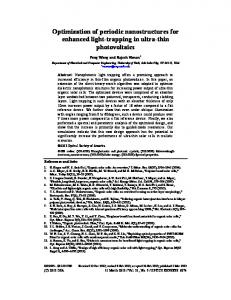
1 ǫx (u) ⊗ ǫx (u) dx − |Ke |πΛ Te (y), , (20) |Y | Ke where Te (y) = T(x, y), for x ∈ Ke . Formula (20) defines a scalar function of y which is interpreted as follows. In the perforated cell Y \ Te , the minimum point of (20) is looked for. If the corresponding minimum value is negative, then a small hole is nucleated at that point; otherwise, no action is taken. Figure 6 shows an outline of the algorithm. Figure 7 presents some implementation details. The program has two main components: one of them is a microscopic analysis and optimization code, written in FORTRAN, introduced 11

CONTROL SCRIPT Python homogenized elastic coefficients

sensitivities homogenized elastic coefficients

Z sensitivities

ǫ(u)⊗ ǫ(u)

densities

Ke

optmization parameters

MICROSCOPIC OPTIMIZATION (shape, topology)

MACROSCOPIC ANALYSIS C++ libMesh

FORTRAN

FreeFem++

Figure 7: Data flow diagram in [10] and [9] and improved in [5]. Another component is a macroscopic analysis tool for which we could have used any well-known software, but which we have chosen to implement directly. Two versions have been tested, one of them written in FreeFem++ and the other one written in C++ with the use of the libMesh library. A control script written in Python links these two main components. While the volume of information handled by the microscopic analysis and optimization code is huge, since it deals with a finite element mesh on the periodicity cell for each macroscopic finite element Ke , it only needs to send to and receive from the macroscopic code (through the control script) tiny pieces of information: the homogenized elastic tensor (16 scalar values for each Ke ), the shape/topology sensitivities (32 scalar values for each Ke ), the material densities (one scalar value for each Ke ) and some optimization parameters. Note that, at each optimization step, the treatment of each model hole Te is independent of other model holes, in different zones of the macroscopic body. This is why this problem is well-suited for parallel computation. Several versions of the control script have been tested. Recall that N model holes must be optimized, where N is the number of macroscopic finite elements. A first version of the script launches p simultaneous cellular processes (using the Popen function in the subprocess module of the Python language) and puts them in a queue. When the first process in the queue finishes, the script launches another cellular process. This has the disadvantage that some processes in the queue may finish before the first one, and in this case the machine waits unnecessarily for the first process, thus wasting execution time. This is why the measured speedup for this version of the script is not significant. A second version launches p simultaneous cellular processes, and when any of them finishes, it launches a new process. It uses the select module of Python in order to select a process whose standard output produces information. The speedup of this second version is significant: the execution speed increases about p times if p is less than or equal to the number of processors of the machine. For larger 12

Figure 8: Initial guess p, the speedup is no longer linear and for very large p the speed remains almost constant. A third version of the script connects to several machines and spreads cellular optimization processes, by using a regular internet link and the protocol ssh, through the external modules pexpect and pxssh. The speedup of this third version can be tremendous, depending on the number of machines involved.

6

Numerical examples

In order to illustrate the method, results for three examples are shown. A cantilever is considered, ocuppying a 2 × 1 rectangle, clamped on its left side and subject to loads on its right side. This rectangle is divided in 200 = 20 × 10 Lagrange finite elements of type Q9. The base elastic material C is taken to have Young modulus E = 1 and Poisson coefficient ν = 0.3. More specifically, Cǫ = 2µǫ + λ(trǫ)I2×2 with µ = 0.38461538 and λ = 0.576923. We minimize Φ + ΛV with Φ defined in (8) and V defined in (9). The Lagrange multiplier is always taken as Λ = 133.33333. These values were chosen in order to facilitate the comparison of our results with other results from the literature, particularly from [1] and [11]. The cellular meshes (on the periodicity cell Y ), are composed of triangular Lagrange P 1 finite elements. The number of elements varies during the optimization process around 1000 triangles. The algorithm starts with an initial guess consisting of a periodic microstructure (constant hole T ), shown in Figure 8. The conventions used in this Figure are: in the center, the density of material, θ = 0.9079239, is drawn as a function defined in the macroscopic domain; on both sides, magnifications of the microstructure in 4 chosen points of the body are shown. Starting with this initial 13

111 000 000 111 000 111 000 111 000 111 000 111 000 111 000 111 000 111 000 111 000 111 000 111 000 111 000 111 000 111 000 111 000 111 000 111 000 111 000 111

Lagrangean

200

180

160

140

0

50

100

150

200

1.4 compliance

volume 1.2

40 1 30

0.8

0.6 0

50

100

150

200

0

50

100

150

200

Figure 9: Cantilever with one load in the middle, problem setting and convergence history structure, the shape and topology of the holes T (x) are varied. One topology optimization step is performed after every 20 shape optimization steps. A similar scheme was used with an alternate directions shape/topology optimization algorithm based on level-set techniques in [12]. No penalization of intermediate densities is applied. Each numerical example is illustrated by two Figures. Firstly, Figures 9, 11 and 13 show the configuration of the body, the applied loads, and three graphics representing the evolution of Φ+ ΛV , of Φ and of V , as functions of the number of iterations. Secondly, in Figures 10, 12 and 14 the optimized structure is presented, with the following same conventions as in Figure 8 : in the center, the density of material, θ, is drawn as a function defined in the macroscopic domain (the 2 × 1 rectangle), using levels of grey. Around this central zone, magnifications of the microstructure in 8 chosen macroscopic finite elements are shown. Note that the homogenized tensor CH of the optimized structure is difficult to represent, since it involves 6 scalar functions. A dynamic version of these Figures is available at [13]. In the first example, a load of intensity 1 is applied in the middle point of the right side of the cantilever. Figure 9 shows the setting of the problem and the evolution of the Lagrangean Φ + ΛV , of the compliance Φ and of the volume of material V , as functions of the number of iterations. It can be seen that the decrease of the Lagrangean is rather slow; this is due to the fact that a very simple minimization algorithm was used (steepest descent). Note that we have

14

a

h

b

g

c

d

e

f

Figure 10: Cantilever with one load in the middle, optimized structure no information on the second derivatives of the functionals involved. Probably, the speed of convergence could be improved by using a quasi-Newton algorithm. In Figure 10, the optimized structure is represented. Note that the algorithm is not allowed to eliminate completely the material from a certain zone, nor to cut completely the material into layers (since this would produce a degenerate homogenized elastic tensor CH ). Thus, the minimum percentage of material allowed is about 9% and is attained by very thin truss-like structures (zoom h). In certain zones, it can be seen that the algorithm produces periodic microstructures close to rank-1 laminates (zooms a and e) or to rank-2 laminates (zooms c and g). Note that there is a known theoretical optimal structure predicted by the theory of homogenization, made of rank-2 laminates; see [14]. In the second example, a load of intensity 1 is applied in the lower right corner of the rectangle, see Figure 11. The optimized structure is represented in Figure 12. One can recognize the appearence of the classical solution. Zoom a corresponds to a zone with full material (density θ = 1): the algorithm is allowed to eliminate completely the model hole. It is noticeable how the microstructures orient themselves in the direction of the principal stress (zooms b, c, e, g). Some of the microstructures (e.g. zoom e) ressemble the Vigdergauztype microstructures, see [15]. As explained in Remark 5, the approach presented here is not limited to the minimization of the compliance: other, more complicated, functionals can be dealt with. The third example involves a multi-load situation. Three loads are considered, as shown in Figure 13, acting independently of each other. The objective functional is the average of the three compliances (for the three load

15

111 000 000 111 000 111 000 111 000 111 000 111 000 111 000 111 000 111 000 111 000 111 000 111 000 111 000 111 000 111 000 111 000 111 000 111 000 111 000 111

Lagrangean 200

180

160

140 0

100

200

300

400

500

600

1.4 volume

45 1.2 40 compliance

1

35 0.8

30 0

100

200

300

400

500

600

0

100

200

300

400

500

600

Figure 11: Cantilever with load in the lower corner, problem setting and convergence history

a

h

b

g a

c

e

d

f

Figure 12: Cantilever with load in the lower corner, optimized structure

16

111 000 000 111 000 111 000 111 000 111 000 111 000 111 000 111 000 111 000 111 000 111 000 111 000 111 000 111 000 111 000 111 000 111 000 111 000 111

Lagrangean 190

170

150

130 0

40

100

300

volume

1.3

35

200

1.1 convex combination of compliances

30 0.9 25 0.7 20

0

100

200

300

0

100

200

300

Figure 13: Cantilever with three independent loads, problem setting and convergence history

a

h

b

g

c

d

e

f

Figure 14: Cantilever with three independent loads, optimized structure

17

cases) : Φ 1 + Φ2 + Φ3 3 The optimized structure is shown in Figure 14. Note that, for this multiload objective functional, there is no guarantee that an optimal structure can be obtained by using rank-two laminates, see [14]. This is confirmed, to a certain extent, by the fact that, in the structure represented in Figure 14, more oval-shaped holes appear in comparison with the two previous examples. These microstructures are supposed to resist well to three different stress states. No symmetry is imposed in the above three examples, either on the macroscopic solution or on the microstructures. In the first and third examples, the macroscopic solution is almost symmetric, as expected. By using a finer macroscopic mesh, we expect to obtain a more perfect symmetry. The authors believe that the solutions could be improved by allowing the periodicity cell to vary during the optimization process, see Remark 3. The evolution of the periodicity cell in each (macroscopic) finite element should be independent of the evolution of the other cells. This would give the microstructures the freedom to orient themselves better; the variation of the periodicity cell should follow the derivative of the objective functional with respect to the vectors defining the periodicity. Φ=

7

Conclusions and future work

The present paper presents an algorithm for the optimization of bodies having locally periodic perforations. Shape and topology optimization steps are performed following an alternate directions approach. The scripting language Python was used in order to launch in parallel cellular optimization processes. Our approach is related to free material optimization in the sense that it uses the derivative of the objective functional with respect to the homogenized elastic coefficients. The method is general : any objective functional can be treated, as long as its derivative with respect to the macroscopic material coefficients can be computed. The numerical results are encouraging, showing good agreement with results from the literature. The upgrade of the algorithm to three-dimensional problems is the object of on-going work. The main difficulty is the implementation of the finite element mesh on the cube with its opposite faces identified (which is equivalent to meshing the three-dimensional torus), especially its deformation and regeneration. Robust algorithms for mesh deformation and mesh regeneration in R3 are difficult to find. Other directions for improving the algorithm in the future are: the implementation of a quasi-Newton algorithm in order to accelerate the convergence and allowing the periodicity cell to vary along the optimization process.

18

Aknowledgements This work was supported by Funda¸ca˜o para a Ciˆencia e a Tecnologia, Financiamento Base 2008 - ISFL/1/209. Paulo Vieira helped with the implementation of the macroscopic analysis code in C++, using the finite element library libMesh. S´ergio Lopes implemented the macroscopic analysis code in FreeFem++. The authors have used the open-source softwares xd3d, xgraphic, by Fran¸cois Jouve, and xfig for graphic creation.

References [1] G. Allaire, Shape Optimization by the Homogenization Method, Springer, Applied Mathematical Sciences 146, 2002 [2] F. Murat, L. Tartar, H-convergence, in: Topics in the Mathematical Modelling of Composite Materials, edited by A. Cherkaev and R. Kohn, Progress in Nonlinear Differential Equations and Their Applications, vol. 31, p. 21-43, Birkh¨ auser, 1997 [3] D. Cioranescu, J.S.J. Paulin, Homogenization in open sets with holes, Journal of Mathematical Analysis and Applications, 71(2), p. 590-607, 1979 [4] C. Barbarosie, A.-M. Toader, Shape and Topology Optimization for periodic problems, Part I, The shape and the topological derivative, Structural and Multidisciplinary Optimization, Online First, DOI 10.1007/s00158-009-03780, 2009 [5] C. Barbarosie, A.-M. Toader, Shape and Topology Optimization for periodic problems, Part II, Optimization algorithm and numerical examples, Structural and Multidisciplinary Optimization, Online First, DOI 10.1007/s00158009-0377-1, 2009 [6] C. Barbarosie, A.-M. Toader, Optimization of bodies with locally periodic microstructure, IRF’2009 Third International Conference on Integrity, Reliability and Failure (Symposium V, Structural and Multidisciplinary Optimization), Porto, 20-24 July 2009 [7] P.G. Coelho, P.R. Fernandes PR, J.M. Guedes, H.C. Rodrigues, A hierarchical model for concurrent material and topology optimisation of threedimensional structures, Structural and Multidisciplinary Optimization, 35(2), p. 107-115, 2008 [8] M.P. Bendsøe, Optimization of Structural Topology, Shape, and Material, Springer, 1995 [9] C. Barbarosie, Shape optimization of periodic structures, Computational Mechanics, 30, p. 235-246, 2003 19

[10] C. Barbarosie, Optimization of perforated domains through homogenization, Structural Optimization, 14(4), p. 225-231, 1997 [11] F. Jouve, private communication, 2009 [12] G. Allaire, F. de Gournay, F. Jouve, A.-M. Toader, Structural optimization using topological and shape sensitivity via a level set method, Control and Cybernetics 34, p. 59-80, 2005 [13] http://cmaf.ptmat.fc.ul.pt/~barbaros/en/examples-2009.html (web page) [14] G. Allaire, R.V. Kohn, Optimal design for minimum weight and compliance in plane stress using extremal microstructures , Europ. J. Mech. A/Solids 12, 6, p. 839-878, 1993 [15] S. Vigdergauz, Two-dimensional grained composites of minimum stress concentration, International Journal of Solids and Structures, 34 (6), p. 661-672 (1997)

20