Optimization of cost functions in ATPDraw Hans Kristian Høidalen NTNU, Norway
Electric Power Engineering / NTNU O.S. Bragstadspl. 2F N-7491, Trondheim, Norway +47 73594225/Fax:73594279
[email protected]
Daniel Radu Schneider Electric, France
R&D Department 31, rue Pierre Mendes France 38050, Grenoble Cedex 9, France
[email protected]
Delcho Penkov Schneider Electric, France
Power Systems 20, av. des Jeux Olympiques 38100, Grenoble, France
[email protected]
Abstract - The paper outlines a family of new options in ATPDraw to facilitate optimization of circuit parameters. This consists of a new approach for $Parameters using intermediate variables, special ATPDraw syntax to control variables as a function of the simulation number (KNT), a new Models component used for writing extreme values to and reading from the lis-file, and three algorithms used for constrained optimization of multiple circuit variables. A new example circuit in ATPDraw studying resonance grounding of a 24 kV power systems is introduced. The family of new components and solutions is used to view the resonance curve and automatically tune the neutral inductor to resonance. As a second example the initialization of two type 59 synchronous machines is shown. The last case study deals with the sizing of medium voltage circuit breaker protections, to control the Transient Recovery Voltage. Keywords: ATPDraw, Optimization, Genetic Algorithm, Gradient Method, Simplex Annealing, Resonance grounding, synchronous machine initialization, load flow, TRV.
1 Introduction Optimization was during the last decades one of the most discussed topics, the continuous evolution of the optimization techniques being conducted by the extension of the problems to be solved. Defined as the process of finding the conditions that give the minimum or maximum value of a function, where the function represents the effort required or the desired benefit, the optimization has a large panel of applications. Hence, we will find them as an important tool in the power systems analyses. In the electromagnetic transient analyses field, the
optimization of circuit parameters for tuned design and performance has been reported in the literature and implemented in PSCAD [1, 2]. Large number of optimization methods coexists, according to the type of the problem; constrained or not, continuous or discrete, etc… Among these optimization methods, several heuristic tools have evolved, that facilitate the solution of optimization problems that were previously difficult or impossible to solve. Hence, we can find: evolutionary computation, simulated annealing, taboo search, particle swarm, etc., the major advantages consisting in a development time that is much shorter than when using more traditional approaches, and, in a very robust system which is relatively insensitive to noisy and/or missing data. Three different optimization methods are investigated in this paper: Gradient Method (GM) (Quasi-Newton, BFGS) and two meta-heuristic methods: Genetic Algorithm (GA) and Simplex Annealing (SA). Gradient based methods are good at arriving at local minima quickly, but might fail to obtain global solutions. Such methods also have difficulties with rough surfaces which typically can be the case in situations with numerical round-off errors. On the other hand a Genetic Algorithm is typically good at obtaining a global minimum. The process is however slow and the exact solution is seldom found. The Simplex Annealing method is based on the Nelder-Mead algorithm with a random tolerance given by the simulated annealing process. This method can theoretically, if parameters are tuned properly, handle rough surfaces, local minima and arrive at exact solutions. The paper first explains the implementation of the various required elements. Then the examples that illustrate the new options are presented.
2 Implementation The implementation of optimization uses the $PARAMETER option in ATP with PCVP in order to achieve a faster calculation. In the implementation of the GA up to twenty cost function evaluations are performed and in the case of GM two times the number of variables plus one with one ATP call. It was thus required to considerably revise the implementation of $Parameter in ATPDraw version 5.6. Next, a general purpose cost function had to be included. Finally, an Optimization dialog is introduced that performs the actual ATP file handling and optimization routine execution. The optimization problem is defined as the minimization or maximization of the object function OF in n dimensions with variables x.
max OF ( x1 , x2 ,… , xn ) min The variables x are can be selected by the user among the global variables. A) Optimization routines The Gradient Method (GM) is the L-BFGS-B routine [3] (limited memory algorithm for bound constrained optimization) which is a quasi-Newton method with numerical calculation of the gradient. The gradient is calculated based on the two point formula:
∂f f ( x + h) − f ( x − h) ≈ ∂x 2h where the discretization point h is calculated as h = max( x ,10−6 ) ⋅ dx where dx is a user selectable parameter (delta X). If n is the number of variables in the optimization problem the cost function thus has to be evaluated 2n+1 times for each solution point. The iteration number is somewhat loosely defined in the Gradient Method. If the solution is poorer than the previous point the algorithm steps backwards along the gradient until an improved solution is found and only then the iteration number is incremented. The Genetic Algorithm (GA) is based on the RiverSoft AVG package (www.RiverSoftAVG.com), but modified to better handle the variable constraints. This optimization routine might need further improvement and development. The evolvement of the solution with GA is to more or less randomly select solutions (individuals) and mate these to obtain new solutions. The selection process can be Random, Roulette (using cumulative distribution), Tournament (competition between a user selectable number of randomly selected rivals), Stochastic Tournament (combination of Roulette and Tournament), and Elitism (select only the user defined best percentage of the population). Tournament with 5-10 rivals is a reasonable starting point. The user has to select the size of the population (maximum 1000) and this is a critical parameter which depends on the problem and the number of variables. The user must also select the resolution with 8, 16 and 32 bits available. This part needs further development to allow integer values and arbitrary resolutions. The Simplex Annealing (SA) method is implemented from [4]. It is based on the NelderMead simplex algorithm with an added random behaviour gradually reduced (simulated annealing). The algorithm also uses a possible larger set of points (called population) and can support mutation. With all control parameters set to zero the algorithm simply reduces to the classical Nelder-Mead simplex method used in [1, 2]. The method relies only on function evaluations and POCKET CALCULATOR of ATP is thus not used. Since a single case is run through ATP for each cost function evaluation, the method thus has potential to be extended to include other variables than those defined within the global variables ($Parameter). B) $PARAMETER The concept of Variables was introduced in ATPDraw 3.0 and is significantly updated in version 5.6. The user is allowed to specify a 6-character text string instead of a data value in the component dialog box. A value is then assigned to this text string under the Variables tag of the ATP|Settings dialog box as shown in Fig.1. In order to allow a variable for the data value its Param property must be set to unity under Edit Definitions/Data. In cases where the data value is used in calculations in the component (for instance the phase angle of a 3-phase AC source) variables are not allowed and the default value is in such cases used instead. Variables are also allowed for Models. If the Number of simulations is larger than unity a POCKET CALCULATOR VARIES PARAMETERS card is inserted and the simulation is
repeated this number of times. The current simulation number is then available as the parameter 'KNT'. The variables specified by the user appear to the left and the user has to assign values for the variables. This is done in free format in the column to the right in Fig. 1. All the variables are declared as intermediate and the flag '$$' is automatically added at the end. The variables used in the circuit are then assigned to these variables and ATPDraw automatically adds underscore characters to obtain the maximum resolution. A variable 'RES' used for both high and low precision resistances will thus be repeated twice (highest precision declared first) with 13 and 3 underscore characters added, respectively. The intermediate variable is renamed 'RESI' (character 'I' for intermediate added). This process is hidden, however, but the result is seen in the final ATP file under the $Parameter declaration. The user can also define local, intermediate variables. The user should not use underscore characters in the name of variables. Examples of input of variables are shown in Fig. 1. All variables are declared as intermediate so that referencing is allowed. The variable MYVAR must be declared before RES which must come in front of CAP. The resulting $PARAMETER cards in the ATP file are shown below Fig. 1. IMPORTANT! Since only floating point numbers are supported by ATP always use a period '.' after a number in the value field.
Fig. 1. Specification of variables where the last three are linked to component data.
The specification in Fig. 1 will produced the following ATP file format: $PARAMETER F01001=(KNT.EQ.1.)*2.3 $$ {Special outcome of the '@[' or '@FILE' specification: F01002=(KNT.EQ.2.)*4.6 $$ {Fyyxxx: F=Factor, yy=array number, xxx=index number. F01003=(KNT.EQ.3.)*5.3 $$ F01004=(KNT.EQ.4.)*2. $$ F01005=(KNT.GE.5.)*3.1 $$ MYVARI=F01001+F01002+F01003+F01004+F01005 $$ {Variables Pyyzzz are introduced if more than 9 items RESI =4.5*MYVARI $$ {'I' added to 'RES' to mark intermediate variable name CAPI =12.3/RESI*KNT $$ {RESI automatically substituted for RES here. KNT=Simulation number 1..5 MODVARI =2.3 $$ {Simple/Normal value assignment RES_____________=RESI {High precision RES declared first RES___=RESI {Low precision RES comes next MODVAR__=MODVARI {Model data variable 8-character default resolution, modify the Digits property. CAP_____________=CAPI {High precision capacitance BLANK $PARAMETER
Several special new features are introduced in ATPDraw 5.6. MyVar=@[a b c d e f g] The characters '@[' are used to identify this format. Space or comma can be used to separate the numbers (integer or floating point). First run (KNT=1): MyVar=a Second run (KNT=2): MyVar=b ... Seventh run and beyond (KNT >=7): MyVar=g, etc. MyVar=@FILE FileName Col '@FILE' is the keyword, FileName is the name of a text file assumed stored in the ResultDirectory (same as final ATP file) (enclose the file name within " " if it contains space), and Col is an optional parameter identifying which column in the text file to use. The text file can have integer or floating point values in free format, space or comma separated: 34.5, 45.234567 1.23e-3 2 3, 4 If Col is not specified the first column of the file is loaded. The length of the file does not need the match the chosen Number of Simulations. First run (KNT=1): MyVar=First value of column Col (Col=2 -> 45.234567) Second run (KNT=2): MyVar=Second value of column Col (Col=2 -> 3.0) etc.
Both the '@[' and '@FILE' syntax rely on the same implementation and requires a lot of intermediate variables. There seems to be a limit in ATP of 60 intermediate variables. It might be possible to increase this limit using the INDOFF variable as illustrated in benchmark DCN19.dat. MyVar=@LIN Lo Hi '@LIN' is the keyword. Create a linear space. MyVar=a*(KNT-1)+b MyVar=@LOG Lo Hi '@LOG' is the keyword. Create a logarithmic space. MyVar=10**(a*(KNT-1)+b) MyVar=@POW Lo Hi P '@POW' is the keyword. MyVar = a*(KNT-1)**P+b MyVar=@EXP Lo Hi P '@EXP' is the keyword. MyVar = a*P**(KNT-1)+b If P ='e' this is replaced by exp(1).
a and b are calculated based on Lo and Hi: First run (KNT=1) MyVar=Lo, Last run (KNT=Number of Simulations) MyVar=Hi. This last four options could easily be managed directly be the user. The Optimization module lets the user choose the variables as specified under NAME in Fig. 1. In such case the right VALUE field is ignored and overwritten. The Optimization module takes advantage of the @FILE option.
C) Cost function A general purpose Cost Function in MODELS called WRITEMAXMIN is introduced in ATPDraw version 5.6. The idea is to extract a single value from a simulation and write this to the lis-file and read it back when the simulation is finished. The single value is either the maximum or minimum of the signal xout from time Tlimit and out to the end time of the simulation. The Model has one input but this can be expanded. The Model also takes in one DATA parameter AsFuncOf and if this is assigned to a variable WRITEMAXMIN writes output as function of this data parameter. If AsFuncOf is a number it is simply replaced by the simulation number. WRITEMAXMIN supports multiple run though POCKET CALCULATOR. The selection of the component and its input dialog is shown in Fig. 2. The WRITEMAXMIN component can be used also in other cases than Optimization as illustrated later.
Fig. 2 Cost Function WRITEMAXMIN.
D) Optimization dialog The Optimization dialog is found under ATP|Optimization. The user has to set up the data case which is not stored with the project. The variables x1..xn are chosen by clicking in the Variables column and selecting the available variable in the appearing combo box as shown to the left in Fig. 3. The user also has to specify the constraints Minimum and Maximum. The Object function must be selected among the available WRITEMAXMIN components in the circuit. The user can then select to minimize or maximize and select a solution method (Genetic Algorithm, Gradient Method or Simplex Annealing). The Max iter field is the maximum number of iterations in the solution algorithm. For the Genetic Algorithm there are several, special selections. The size of the Population is a critical parameter. A low number will produce a degenerated result, while a too high number will waste computation time. The maximum allowed number is 1000. The required Resolution depends on the selected range (Max-Min). Since it anyhow is recommended to switch to the Gradient Method for fine tuning a 8-bit resolution (255 steps) is normally sufficient. The
Population count and Resolution can not be changed in the optimization process (Continue). The Crossover probability should be set to a high number (


![Cost Optimization Pillar [PDF]](https://m.moam.info/img/260x300/cost-optimization-pillar-pdf_6479b31b098a9e2a3a8b457b.jpg)