IEEE TRANSACTIONS ON IMAGE PROCESSING, VOL. 14, NO. 11, NOVEMBER 2005
1831
Optimization of Integer Wavelet Transforms Based on Difference Correlation Structures Hongliang Li, Guizhong Liu, and Zhongwei Zhang
Abstract—In this paper, a novel lifting integer wavelet transform based on difference correlation structure (DCCS-LIWT) is proposed. First, we establish a relationship between the performance of a linear predictor and the difference correlations of an image. The obtained results provide a theoretical foundation for the following construction of the optimal lifting filters. Then, the optimal prediction lifting coefficients in the sense of least-square prediction error are derived. DCCS-LIWT puts heavy emphasis on image inherent dependence. A distinct feature of this method is the use of the variance-normalized autocorrelation function of the difference image to construct a linear predictor and adapt the predictor to varying image sources. The proposed scheme also allows respective calculations of the lifting filters for the horizontal and vertical orientations. Experimental evaluation shows that the proposed method produces better results than the other well-known integer transforms for the lossless image compression. Index Terms—Difference correlation structure, integer wavelet transform, lifting scheme, lossless compression.
I. INTRODUCTION
T
HERE HAS been a growing interest in integer-to-integer lifting wavelet transforms for image coding applications [1]–[23]. Due largely to the better computational efficiency and to the fact of providing a new method for filter design, transforms of this type are extremely useful for compression systems requiring efficient handling of lossless coding, and minimal memory usage [9]. Such transformation is a basic modification to the linear transforms, where each filter output is rounded to the nearest integer, which reduces the costly floating point operations. The transform coefficients show the feature of being exactly represented by finite precision numbers, which can be used for truly lossless encoding [1], [3]. The reversible integer-to-integer wavelet transforms considered in this study are based on the lifting framework [1] and are constructed using the technique described in [3]. The fundamentals of lifting can be found in [1]–[7]. An algorithm for decomposing wavelet transforms into lifting steps was described in [6]. Some nonlinear wavelet transforms were also recently investigated in [24]–[30]. Calderbank et al. [3] presented two approaches that lead to wavelet transforms that map integers to
Manuscript received May 30, 2003; revised September 9, 2004. This work was supported in part by the China National Natural Science Foundation (CNSF) under Project 60272072, by the Ministry of Education of China Trans-Century Elitists under Project TCEP, 2002, and by the Ministry of Education of China under “The Tenth Five Years Plan”/“211”project at Xi’an Jiaotong University. The associate editor coordinating the review of this manuscript and approving it for publication was Dr. David S. Taubman. The authors are with the School of Electronics and Information Engineering, Xi’an Jiaotong University, Xi’an 710049, China, (e-mail: hlli@ mailst.xjtu.edu.cn;
[email protected];
[email protected]). Digital Object Identifier 10.1109/TIP.2005.854476
integers. The first approach exploits the precoder of Laroia et al. [8], which is integrated with expansion factors for the high and low pass band in subband filtering. The second approach builds upon the idea of factoring wavelet transforms into lifting steps, and looks more promising for lossless image coding. In order to evaluate the effectiveness of various wavelet filters for lossless compression of digital images, a set of test images including natural images, computer-generated images, compound images and different types of medical images were used in [3]. All of these images were compressed in a lossless manner using the various transforms under evaluation. Similar performance and more filter evaluation can also be found in [9]–[11]. Both studies [3], [9] declare that there is no filter that consistently performs better than all the other filters on all the test images. In order to find optimal lifting coefficients (i.e., the coefficients of lifting filters) for lossless image compression, Yoo and Jeong [12] utilize an exhaustive search in the experiment. The lifting coefficients which gave the minimum weighted first-order entropy are adopted by varying the prediction coefficients from 0 to 32 and update coefficients from 0 to 16, respectively. Boulgouris et al. [13] first calculate the optimal predictors of a lifting scheme in the general -dimensional case and then apply these prediction filters with the corresponding update filters to the lossless compression of still images using first the quincunx sampling and then the simple row-column sampling. In each case, the linear predictors are enhanced by a directional nonlinear postprocessing in the quincunx case, and then by 6, 4, and 2 vanishing moments nonlinear postprocessing in the row-column case. In order to achieve this, the resulting six predictions are ordered according to their magnitudes and the average of the third and fourth is then taken as the prediction. Grangetto et al. [14] propose several methods for the selection of the best factorizations of wavelet filters within the lifting scheme framework. The methods are based on the search for the minimally nonlinear iterated graphic functions [15] associated to integer transforms and on the minimization of the number of lifting steps. Taubman [16] develops adaptive wavelet transforms to modify the prediction step by exploiting local orientation information at edge boundaries. Moreover, Claypoole et al. [17] use lifting to design customized DWTs that adapt to the signal under consideration.They perform the space-adaptive transforms by choosing the order number from {1,3,5,7 } that minimizes the prediction values. Recently, Deever and Hemami [18] developed a projection technique that is used to derive optimal final prediction steps for lifting-based reversible integer wavelet transforms. Using this method, a transform basis vector is projected onto a subspace spanned by neighboring (sharing some spatial support) basis vectors
1057-7149/$20.00 © 2005 IEEE
1832
IEEE TRANSACTIONS ON IMAGE PROCESSING, VOL. 14, NO. 11, NOVEMBER 2005
to derive precise projection coefficients that can be used in an additional lifting step. In this paper, we address the issue of dynamic calculation of the optimal predictors in the sense of minimizing the prediction error variance which has a similar objective as the method by Boulgouris et al. [13]. In that work, the optimized predictors are derived in transform domain. As before, it is necessary to specify appropriate spectral density models describing the class of original images which are of interest. Based on the assumed density model, the optimal prediction filter can be determined. In our work, however, a new idea based on the difference correlation structure (DCCS) is presented for finding the optimal lifting coefficients. The impact of the difference correlation function on the linear predictor is firstly investigated. Then, based on the lifting scheme, the effective prediction and update coefficients are derived in terms of the correlation functions. Unlike the traditional lifting schemes, the proposed method puts heavy emphasis on the inherent difference correlation feature for each image. We compare the optimal lifting filters to the existing well-known lifting wavelet filters, showing that in most cases reduced entropies and final bitrates can be achieved for various content images. This paper is organized as follows. The impact of the first and the second-order correlation functions of difference images on the linear predictors will be analyzed in Section II. In Section III, the newly proposed methods for calculating the optimal lifting filters are described, and results are given. Experimental results are provided in Section IV to support the efficiency of the new lifting filters. Finally, in Section V, conclusions are drawn and further research proposed. II. IMPACT OF THE DIFFERENCE CORRELATIONS ON THE LINEAR PREDICTOR In this section, we will investigate the impact of the variancenormalized autocorrelation function of the difference image on the linear predictor, which may provide the foundation for the following lifting filters construction. First, let us consider an image in which each pixel is in turn mapped onto a point on the actual surface. The gray level corresponds to the quantity of secondary electrons being emitted from that point. According to Kretzmer’s experiment [31], the amplitude difference between the adjoining pixels is close to zero. The result implies that the brightness level at a point in an image is highly dependent on the brightness levels of its neighboring points unless the image is simply a random noise. The corresponding Markov random field (MRF) model of this dependence has been investigated in [32]–[36] for a long history. In this model, the image region is described as a sample realization of a random field, usually isotropic and homogeneous, and with significant correlations well beyond nearest neighbors. The density of a pixel at a certain location is only determined by its neighbors. Although the correlation properties of different images have been widely studied in the literature, at present, fewer works relevant to the dependence properties of the difference images have been reported, especially for the issue of their impact on the linear predictors. As one might expect, the image content
is an important factor influencing the effectiveness of the linear prediction. The prediction process can also be described as the decorrelation process, which is reducing the spatial correlation among the adjacent pixels of the original image. Let us concentrate now on a linear predictor to perform the decorrelation process. Since the image is handled by transforming the rows and columns in succession, the transforms under consideration are one-dimensional (1-D) in nature. be a 1-D signal of inteWithout loss of generality, let . In our study, we usually assume the gers has enough samples ( ), whose effect discrete signal on the calculation of the autocorrelation can be neglected. Its , variance-normalized autocorrelation function at lag by is given as follows: (1) where (2) We define the first and the second-order difference signals, respectively, by (3) and (4) The corresponding variance-normalized autocorrelation functions can be written as
(5)
(6) Moreover, suppose and denote the height and width of an image, respectively. The horizontal and vertical variance-normalized autocorrelation of the image are, respectively, calculated by (7)
LI et al.: OPTIMIZATION OF INTEGER WAVELET TRANSFORMS
1833
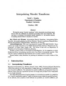
Fig. 1. First row: Three test images (sar1, hotel, finger2). Second row: Horizontal variance-normalized autocorrelation functions for the original. Third row: First-order difference. Final row: Second-order difference images.
(8)
where
(9)
It is worth noticing that correlation structures are an inherent image characteristic. Many images, which exhibit the same correlation properties, might differ from each other according to their DCCSs. In order to address this issue, three test images
(sar1, hotel, finger2) with their respective horizontal variance-normalized autocorrelation coefficients computed from (7), are presented in the first and the second rows of Fig. 1. Their corresponding horizontal variance-normalized autocorrelation coefficients of the first and the second-order difference images are given in the latter two rows. As shown in Fig. 1, although all of them exhibit high correlation in the original images, obvious discrepancies of the correlation properties can be observed in the difference images. For example, from left to right, the correlation coefficients of the first-order difference images are increasing gradually. The corresponding one-step horizontal correlation coefficients are equal to 0.1879, 0.2803, and 0.7506, respectively. For the second-order difference images, only finger2 exhibits higher correlation characteristic (about 0.5196).
1834
IEEE TRANSACTIONS ON IMAGE PROCESSING, VOL. 14, NO. 11, NOVEMBER 2005
Now, let us consider the case of the difference signal without any autocorrelation. In other for all . Then, from (5), words, we assume that we have
In the notation of the variance-normalized autocorrelation function, (14) can be rewritten as (15) See the equation at the bottom of the page. Substituting the derived relation (11) into the above equation for , we obtain (16)
(10)
where
Using the recursive process, we can rewrite (10) as
.. .
.. .
.. .
.. .
.. .
.. .
.. .
.. .
.. .
.. .
.. .
.. .
.. .
.. .
.. .
.. .
.. .
.. .
.. .
.. .
.. .
.. .
.. .
.. .
.. .
.. .
.. .
.. .
(11) th-order Suppose we only investigate the construction of a linear predictor without the consideration of the even and odd , namely sampling process for a 1-D signal
(12)
are
the prediction coefficients satisfying . The optimal coefficients are those which result in the least-square prediction error between and , i.e., the quantity where
Then, the optimal coefficients are given by (17)
(13)
Using the knowledge of matrix analysis, we can easily derive the corresponding inverse matrix and rewrite (17) as is minimized. Since is a quadratic function, it has a unique that minimize are found minimum. The coefficients by taking the gradient, setting it equal to zero and then solving the following system of linear equations for
.. . (18) .. .
(14)
.. .
.. .
.. .
.. .
.. .
.. .
.. .
.. .
.. .
.. .
.. .
.. .
.. .
.. .
.. .
.. .
.. .
.. .
LI et al.: OPTIMIZATION OF INTEGER WAVELET TRANSFORMS
1835
See the equation at the bottom of the page. Here, the dashed line indicates that the upper parts in maand have the same dimensions. Thus, for trices , we can obtain the optimal coefficients (18), as follows:
See the equation at the bottom of the next page. Thus, using the same approach as (18), for , we have
(23) (19) Next, we consider the case of the second-order difference signal with the form (4). Suppose that the variance-normalized autocorrelation functions of the second-order difference signal . Then, from (6), are identically equal to zeros except at we have
Furthermore, if the second-order difference signal still has strong correlation, and the third-order variance-normalized autocorrelation functions are equal to zeros except at , the optimal coefficients turn out to be
(24) (20) where
(21) The optimal coefficients, namely the solutions to (15), can now be written as (22)
.. .
.. .
From the above analysis, we can see that the prediction order of the linear predictor depends highly on the difference correlation function of the test signal. For those signals with small first-order difference correlation, the two-tap predictor should be considered. As for the case with small second-order difference correlation, the corresponding four-tap linear predictor should be employed. Similarly, the six-tap predictor performs better than the others if the signal exhibits very small variancenormalized autocorrelation in the third-order difference image. These results motivate us to reasonably assume that the lifting filters coefficients may be efficiently represented by the difference correlation functions.
.. .
.. .
.. .
.. .
.. .
.. .
.. .
.. .
.. .
.. .
.. .
.. .
.. .
.. .
.. .
.. .
.. .
.. .
.. .
.. .
.. .
.. .
.. .
.. .
.. .
.. .
.. .
.. .
.. .
.. .
.. .
.. .
.. .
.. .
.. .
.. .
1836
IEEE TRANSACTIONS ON IMAGE PROCESSING, VOL. 14, NO. 11, NOVEMBER 2005
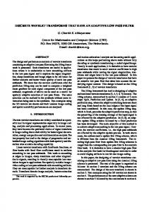
Fig. 2. Basic forward lifting wavelet transform. P and U stand for the prediction and update lifting operators, respectively.
III. DCCS-BASED LIFTING INTEGER WAVELET TRANSFORMS
split into two signals corresponding to evenly and oddly indexed samples. Then, a lifting filter is applied to one of the samples signal and the results are used to subtract from the other one. Eventually, after several lifting steps, the two samples will be replaced by the low pass and high pass coefficients, respectively. As described in the block diagram of Fig. 2, the prediction stage uses the even samples to predict the odd ones in terms of a predict filter, while the update stage consumes the samples produced in the prediction stage to update the current phase and produces as such a low-pass coefficient. Using eight discrete points, the lifting process with four-tap predictor is depicted in Fig. 3. Here, the filter coefficients are supposed to be symmetric. We use
The preceding section was devoted to the impact analysis of the difference correlation on the linear predictor. In this section we shall address the construction of the optimal lifting filters based on the DCCS. A. Lifting Scheme for Integer Wavelet Transforms As mentioned earlier, the lifting scheme presented by Sweldens [1], [2] allows the new integer wavelet transform, which can be used to realize a unified lossless codec. The basic lifting scheme comprises several stages: first, the input data are
.. .
.. .
.. .
.. .
.. .
.. .
.. .
.. .
.. .
.. .
.. .
.. .
.. .
.. .
.. .
.. .
.. .
.. .
.. .
.. .
.. .
.. .
.. .
.. .
LI et al.: OPTIMIZATION OF INTEGER WAVELET TRANSFORMS
1837
Fig. 3. Example of the lifting wavelet transform with eight discrete points. d and x denote the high- and low-pass coefficients, respectively. represent the prediction coefficients, while q and (1=4) + q denote the update coefficients.
0
and
to denote the prediction coefficients, and and to stand for the update coefficients. If the prediction and update coefficients are equal to the fixed values, several well known lifting filters can be obtained. For example, the filter coand are used to perform the simple efficients with 5/3 transform. More conventional filters can be found in [3], [4], [9], and [22]. In the evaluation of integer wavelet transforms [9], it was presented that, for the natural images, the 5/11-C, 5/11-A, and 13/7-T transforms generally perform best, followed closely by the 9/7-M and 13/7-C transforms. For images with a relatively greater amount of high-frequency contents, the 5/3 transform tends to yield the best results often by a significant margin. These results motivate us to use the DCCS to construct a optimized integer wavelet transform capable of better performance for all types of images being transformed.
where symmetric, i.e.,
0p
and (1=2) + p
. Assuming coefficients , we have
are
(26) Let us now return to the problem of determining the optimal lifting coefficients. In our study, we take two cases (namely the lifting wavelet transforms with order 4 and 6) into account. Case I: First, we consider the integer lifting wavelet trans). Let denote the current predicform with order 4 ( tion point. Using the prediction coefficients depicted in Fig. 3, (26) can be rewritten as
B. Lifting Integer Wavelet Transform (LIWT) Based on DCCS Using the predictive lifting format, (12) can be rewritten as follows:
for a certain
(25)
(27) and is given by (28), The prediction error between shown at the bottom of the page. Therefore, the coefficient that minimizes is found by taking the gradient, setting it equal
(28)
1838
to zero and then solving for of the page]. We have
IEEE TRANSACTIONS ON IMAGE PROCESSING, VOL. 14, NO. 11, NOVEMBER 2005
[see (29), shown at the bottom
The second is for the case of sponds to the analysis filter
, which corre-
(30) (33) From the above equation, we can see that the optimal predicwill be close to zero if there exists very low tion coefficient tends correlation in the first-order difference signal, i.e., . This result acts in accord with the preto be zero at lag vious analysis in Section II. In general, the update step should be to smooth even coefficients as much as possible so that they can be easily decomposed in the next decomposition level. Let us now concentrate on the regularity analysis (see [37]–[39]), which can be used to determine the appropriate parameter for the update filter. Using the polyphase matrix given in [37], we can express the analysis filter (low pass) in the domain as
(31) From the above equation, we can see that there exist two special cases that should be considered for the coefficient determination. The first is for the case of , which corresponds to the analysis filter
The factorizations of given in (31)–(33) demonstrate that we have 2, 2, and 4 vanishing moments since there are 2, 2, and in , respectively. 4 zeros at Let us first concentrate on the general case (31). To actually compute the Sobolev regularity, we need to find the transfer operator and its invariant submatrix [37]. Then, we compute the corresponding eigenvalues and obtain the spectral radius of the transition operator. Using the exact computation method for the Sobolev exponent given in [37] and [38], we can easily find the final 11 11 submatrix of the transfer operator with respect to in (31). Since there exist two variables and in this matrix, it is difficult to obtain its eigenvalues with analytical expressions. Fortunately, our goal in this work is mainly concentrated on the determination of the coefficient from the optimal predicrather than the accurate eigenvalues exprestion coefficient sions. Therefore, we can employ the numerical analysis method to study the relation between and . The detailed steps can be equal to which can be described as follows. 1) Let , . 2) For each , we change from 0 to have varied from to 1 with a fixed interval , i.e., with . 3) For each parameter pair , we of the corresponding submacompute the largest eigenvalue , which trix. 4) Finally, we can find the parameter pair has the minimal spectral radius of the transition operator for the . The main reason is that the smaller the spectral coefficient radius of the transition operator, the smoother the scaling function associated with the scaling filter [40]. This also implies that might lead to the better regularity of the analthe coefficient . ysis filter for the prediction coefficient with Fig. 4 shows the actual computation results of , , and . From the obtained result, we can see that a distinct linear relation between and can be observed. Thus, we have the following reasonable assumption: (34)
(32)
Using the linear regression approach, the parameters can be easily computed, i.e., and in our work.
and
(29)
LI et al.: OPTIMIZATION OF INTEGER WAVELET TRANSFORMS
1839
Fig. 4. Numerically determined relationship between p and the q which yields the smoothest scaling function.
Let us now return to the above special cases relative to (32) and (33). Using the similar analysis method as the general case, we compute their maximal Sobolev exponents for each , respectively, and compare the results to that obtained from (31). It is found that, on average, the better regularity can be achieved for (31) with Sobolev exponent increases of about 0.7831 and 0.1702 relative to (32) and (33), respectively. Case II: We now consider the LIWT with order 6 (namely ). Using two prediction parameters, (26) can be rewritten as
(36), shown at the bottom of the page. Thus, the coefficients and that minimize are found by taking the gradient, setting it equal to zero and then solving for them, respectively
(35)
(39)
To optimize the prediction coefficients, we minimize the enand according to ergy of prediction error between
(40)
(37) (38) The corresponding prediction coefficients in (37) and (38) are given by
(36)
1840
IEEE TRANSACTIONS ON IMAGE PROCESSING, VOL. 14, NO. 11, NOVEMBER 2005
(a)
(b) Fig. 5. (a) Relation of q to p for a fixed parameter p = 0:0293. (b) Relation of q to p for a fixed parameter p = 0:0990.
LI et al.: OPTIMIZATION OF INTEGER WAVELET TRANSFORMS
1841
where
TABLE I CONVENTIONAL FILTERS
(41) As for the calculation of the update coefficient for the sixthorder lifting wavelet transform, we still take the similar analysis in the method as the fourth-order case. The analysis filter -domain can be expressed as
(42) The numerical analysis method stated above for the fourth-order lifting transform is also applied to study the relation of to and . Fig. 5(a) shows the actual computation result of and for a fixed coefficient . coefficients for a fixed coefficient Fig. 5(b) shows the relation of and . From the obtained result, we can see that distinct linear relations between to , as well as to can be observed. Thus, we have the following reasonable assumption: (43) change from 0 to 0.2 and from 0 to 0.1. Using the Let , multivariate linear regression approach, the parameters , , and can be easily determined, i.e., , , , and in our work. Finally, using the derived results described in Sections II and III, the determination of optimal filters presented in this paper can be summarized in the following:
for for others for for others
Case I: : Only the first-order difference correlation functions are taken into account for calculating the prediction lifting filters due to the very small correlation level in the second-order difference signal. The prediction and the update lifting coefficients are presented as follows, respectively [see (44) and (45), shown at the bottom of the page]. It can be noticed that several thresholds for determining the coefficients and are used in our work. As for the prediction coefficient , three cases are taken into account. The first deals with the very low difference correlation level, which may be identified if the one-step variance-normalized autocorrelation function of the first-order difference signal is less than an em). The corresponding prediction pirical value (namely should be set to zero. The same decision is also coefficient and applied to the signals with difference correlation . By taking the analysis result in Section II into consideration, for the first-order difference signal with very small , the variance-normalized autocorrelation functions at lag . In fact, for two-tap predictor should be exploited, i.e., the second case in (44), the variance-normalized autocorrelation functions for the first-order difference signal presented in the given conditions still correspond to the lower level. According to the performance of a lot of lossless compression experiments, however, we found that the better results can be achieved for being equal to 0.031 25 instead of the prediction coefficient , zero. For the third case with difference correlation it is shown that there exists relative high correlation level in the first-order difference signal. Thus, the derived prediction coefficient in (30) which is suitable for the four-tap predictor should be employed. In addition, as for the update parameter , we also take three cases into consideration. For the first one, or which we set equal to zero if corresponds to the lower correlation in the first-order difference
or for
and or for
and
(44)
or and
or
and (45)
1842
IEEE TRANSACTIONS ON IMAGE PROCESSING, VOL. 14, NO. 11, NOVEMBER 2005
TABLE II TEST IMAGES WITH THE CORRESPONDING PARAMETERS
signal. For the second one, we use the value of 0.015 625 instead of zero for the coefficient if is satisfied. Certainly, for the others with respect to the larger correlation in first-order difference signal, (34) should be exploited. : The second-order difference correlation Case II: functions are considered for calculating the prediction lifting filters. Two prediction lifting coefficients are, respectively, oband , in which and tained from can be calculated in terms of (39) and (40). The update lifting coefficient is determined by (43). It is important to note that, since the two-dimensional (2-D) transformation is handled by sequentially applying the 1-D decomposition to the columns and rows of a 2-D image, each lifting coefficient should include the horizontal and vertical orientations, which are calculated separately. Unlike the conventional lifting transforms, the filters by which rows and columns are transformed in our scheme are derived according to the different rows and columns correlation properties. That is, the inverse transform must operate on rows and columns in the reverse process using the corresponding coefficients obtained from the forward transform. Without loss of generality, let and denote the horizontal and vertical prediction lifting coefficients, respectively, and
and stand for the corresponding update coefficients. It should be pointed out that a coupled method for the DCCS-LIWT is proposed if the two-tap predictor with coefficients and is determined to perform the lifting wavelet transform in our work. The method aims to reduce the impact of many edges on the autocorrelation of the difference image. It is observed that an image with larger noise or with local smooth areas and many sharp edges is likely to exhibit very small difference correlation. However, the obvious discrepancies between them can be found. In order to avoid large prediction errors in the presence of edges, we propose the following approach based on the median edge detector that is similar to the method in [41] to improve the performance of the lifting wavelet transform with order 2. The determination of such two-tap filter is also the optimal result for the given image using (44). Let be the estimation value of , we have for others (46) where corresponds to downward truncation and (47), shown at the bottom of the next page. It can be seen that the proposed
LI et al.: OPTIMIZATION OF INTEGER WAVELET TRANSFORMS
1843
TABLE III WEIGHT FIRST-ORDER ENTROPY OF THE TEST IMAGES
approach adopts a threshold , which is used to convert the lifting transform into the edge detection mode. This scheme can effectively avoid the influence of sharp edges in the image on the prediction values. In addition, it is worth mentioning that this method should only be applied to the approximate coefficients rather than the detail coefficients in each decomposition level. The similar idea for reducing the edge artifacts in the lifting scheme can be found in [16] and [17], but, in this paper, we only apply this method for the case of two-tap predictor (i.e., and ), which means that the coupled median based nonlinear predictions can be regarded as the postprocessing stage for the DCCS-based integer wavelet transforms. Of course, if the choice of the coupled method is not adopted, the final optimal result for the case of two-tap predictor will be simplified as the 5/3 transform.
IV. EXPERIMENTAL RESULTS In this section, we evaluate the effectiveness of the proposed optimal wavelet filters by coding variety of grayscale images in lossless manner. For the evaluation, we use some images taken from the set of standard ISO test images (download from [42]) and the others selected from the home pages [43] and [44] as our test data listed in Table II. In this set of test images, there are natural images, computer-generated images (“target”), compound images (“cmpnd1,” “cmpnd2,” “library,” and “france”), fingerprint images (“finger,” “finger2,” and “finger3”), synthetic aperture radar images (“sar1” and “sar2”) and different types of medical images (“x_ray,” “cr,” and “us”), etc. These images vary considerably in size and cover a wide variety of content and difference correlation properties. Since the goal of the eval-
if if otherwise
(47)
1844
IEEE TRANSACTIONS ON IMAGE PROCESSING, VOL. 14, NO. 11, NOVEMBER 2005
Fig. 6. Weighted first-order entropy results relative to the best transform for each image.
uations is only to compare the performance of different transforms, the use of tiling is avoided as possible except for cmpnd2 with a tile size of 1280 2298 and ccit1 with the tile size of 1752 2375. For each image, the difference correlation func, , and ) with respect tions at the offset 1 (i.e., to the horizontal and vertical orientations have been calculated and presented in Table II. According to (39), (40), and (43)–(45), the optimal coefficients of the prediction and update lifting filters in the different directions are then computed for each image, which are shown in Table II. It appears that in most cases the four-tap lifting filters are determined as the optimal filters for the following lifting transforms. Only those images, such as “board,” “barb,” “finger2,” “finger3,” “seismic,” and, so on, are required to employ the six-tap lifting filters. Here, the upper part of the fraction for these images in Table II denotes the prediction lifting coefficient , and the lower part indicates the coefficient . From Table II, it can be observed that all the prediction coefficients will not exceed the corresponding coefficients with the same order given in (23) and (24). The main reason can be explained by the correlation characteristics of the image, in which the three-step autocorrelation is generally smaller than the two-step autocorrelation. The upper bound of the prediction coefficients may be referenced from those results. In the evaluation, we decompose each image into a maximum of five scales, and use the weighted first-order entropy [3] as the objective measure. We first compared the proposed method DCCS-LIWT with various well-known wavelet filters listed in Table I. The final weighted first-order entropies of the test images
are reported in Table III. In our experiment, the threshold in (46) is set to be 80 for the noise images such as “sar2,” “us,” and “library,” and ten for others in the case of the prediction coefficients being equal to zeros. As seen from this Table, the proposed method DCCS in almost all cases, leads to better results than all the other methods. For example, as for those images with relatively larger negative first-order difference correlation functions (e.g., “cmpnd,” “target,” “france,” “cr,” etc.), it is found that the proposed method tends to yield the best results than other filters. Similarly, for those images with high second-order difference correlation functions (e.g., “fingerprint,” “seismic,” “board,” and “barb,” etc.), our method also outperforms the (6,2) transform which achieves the best result in the existing methods. In order to provide additional insight into the results of Table III, relative differences were also computed. For each image, the best transform was used as a reference and the relative differences for the remaining transforms were calculated. The relative performance values have been shown in Fig. 6. It can be clearly observed that no single transform among the conventional filters performs best for all the images. A fixed filter may be only suitable for a certain type of images, which can be illustrated from the better transform result of 5/11-C filter for the nature images. However, the proposed DCCS-based lifting wavelet transform can yield the best prediction results for a large number of test images by the dynamic computation of the lifting coefficients. Using the S+P entropy coder [4], we further evaluate the well-known wavelet filters by attaching an entropy coder to present the actual lossless compression rates. The exact bitrates for the test images are reported in Table IV. It is shown that the
LI et al.: OPTIMIZATION OF INTEGER WAVELET TRANSFORMS
1845
TABLE IV LOSSLESS BIT RATE (BITS/PIXEL) FOR INTEGER WAVELET TRANSFORMS
DCCS-based integer wavelet transform consistently outperforms the conventional filters transforms, and the advantage gained in the proposed transform side can be still maintained in a practical coding scenario. Apart from these traditional filters, we also compared the proposed scheme with the other recently proposed integer wavelet transform techniques including projection-based integer wavelet transforms [18], adaptive prediction scheme [13], and nonlinear wavelet transforms [24]. The corresponding lossless bit rates using those methods are presented in Table V. The projection techniques denoted by (2,2)+Proj., S+Proj., and (4,4)+Proj. in this table can be found in (26), (27), and (30) given in [18], respectively. In addition, in order to apply the adaptive nonlinear wavelet transforms [24] for the lossless compression, we choose the 5/3, 9/7-M, and (6,2) filters as the two-tap, four-tap, and six-tap predictors, respectively. The other analysis processes for the nonlinear prediction are the same as [24]. All the presented results in Table V are still based on the S+P entropy coder since we mainly concentrate on the performance of different transforms. As seen from this table, the proposed DCCS-based integer wavelet transform in almost all cases leads to better results than all the other methods. About 0.07 bpp on average can be decreased for lossless bitrate using the proposed method
with respect to the adaptive scheme proposed by Boulgouris et al. [13] which yields the best result among the existing methods. In addition, from Tables IV and V, we can see that, for those images with large correlation in the second-order different signal such as “barb,” “barb2,” “finger2,” “finger3,” “seismic,” etc., the (4,4)+Proj. transform can yield decrease of about 0.04 bpp in the lossless bitrate with respect to (4,4) transform (namely 13/7-T), but more compression bitrates will be required for (4,4)+Proj. relative to the (4,4) to code the medical and compound images which exhibit lower correlation in first-order difference images. As for (2,2)+Proj. transfrom, about 0.0026 bpp decrease on average in the lossless bitrate can be obtained relative to the (2+2,2) (namely 5/11-C) transform for the same set of images. Next, we will concentrate on the computational complexity of the proposed DCCS-based integer wavelet transforms. In our method, the difference images and the autocorrelation statistics should be taken into account in order to obtain the optimal filter coefficients. However, it can be seen that the additional computational load is mainly imposed on the optimization process of the lifting coefficients before the integer wavelet transforms. The filters are derived only for the first decomposition level and applied to all the levels of the wavelet pyramid so as to decrease
1846
TABLE V LOSSLESS BIT RATE (BITS/PIXEL) FOR INTEGER WAVELET TRANSFORMS
IEEE TRANSACTIONS ON IMAGE PROCESSING, VOL. 14, NO. 11, NOVEMBER 2005
is decomposed into a maximum of five scales. In each decomposition level, we, respectively, calculate the prediction and update coefficients using the proposed method. After comparing the obtained weight first-order entropy with that presented in on avTable III, we can see that the performance loss ( erage) is negligible. Additionally, similar case about the change of image statistics can be observed in the choice of the transform sequence for an image. In this paper, we sequentially apply the 1-D decomposition on the rows followed by columns of a 2-D image. Thus, some inevitable changes of image statistics might occur after the first decomposition on the rows. To investigate the effect of the transform sequence on the optimized lifting coefficients, we apply the separable transform to the same test images by using columns followed by rows. It is found that, on average, only about 0.0018 bpp difference between them will be generated for the lossless performance. Finally, we will focus our attention on three filters, i.e., 9/7-M, 13/7-C, and 13/7-T, which have the same prediction coefficients but different update coefficients. From Table IV, it can be seen that 9/7-M transform with the smaller update coefficients tends to yield better compression results than 13/7-C, and 13/7-T for the medical and compound images. However, for nature images with relative larger correlation in the first-order difference signal such as “board,” “boats,” “barb,” “lena,” “gold,” and so on, the 13/7-C and 13/7-T transforms generally lead to the better lossless compression results than 9/7-M. V. CONCLUSION
the computational complexity. From (44) and (45), it is observed that different cases correspond to different computational com, about seven adplexity. For example, for the case of ditions and seven multiplications are required for each sample of the original signal. If the third condition in (44) is satisfied, about 13 additions and 13 multiplications are needed for each sample to perform the optimization of the coefficient . From (34) and (43), we can see that only one and three multiplications are required for the determination of update coefficients . In addition, it should be noticed that the computational complexity in the inverse transforms except for the coupled case (46) can be competitive with the traditional lifting filters, and no additional optimization process is required. Moreover, there are several issues that should be addressed. First, it has been stated that the proposed method employs different filters in the horizontal and vertical directions. Since the image statistics might change after each filtering operation, optimality can be guaranteed only by computing the image statistics in each decomposition level. However, we only use the filters derived in the first decomposition level instead of all the levels of the wavelet pyramid in this paper. In order to study the performance loss due to the adoption of this strategy, eleven test images, i.e., the top six images in Table III, seismic, gold, lynda, sailboats, and lena, are taken into account. Each image
In this paper, the optimal filter coefficients of a lifting scheme were derived from the difference correlation point of view. The basic idea is motivated by the observation that no existing transform performs best for all classes of images due to its fixed filter coefficients. Therefore, dynamic computation of these coefficients is involved, and the most appropriate choice of the transform depends on the different predictor parameters for each given image. Unlike the conventional lifting transforms, the proposed method puts heavy emphasis on the inherent difference correlation feature of an image, and allows respective calculations of the lifting filters not only for varying image sources, but also for the horizontal and vertical directions. Experimental results were obtained by applying the proposed method to a large number of images. It is shown that the proposed DCCSbased LIWT outperforms the other well-known algorithms in the sense of leading to smaller first-order entropies and the lossless compression bitrates. By considering the future work, we can hope to design more effective filters for multistep lifting wavelet transforms. ACKNOWLEDGMENT The authors would like to thank all the anonymous reviewers for the constructive comments and useful suggestions that led to improvement in the quality, presentation, and organization of this paper. REFERENCES [1] W. Sweldens, “The lifting scheme: A new philosophy in biorthogonal wavelet constructions,” in Proc. SPIE Wavelet Applications Signal Image Processing III, vol. 2569, 1995, pp. 68–79.
LI et al.: OPTIMIZATION OF INTEGER WAVELET TRANSFORMS
[2] [3] [4] [5] [6] [7] [8]
[9]
[10]
[11] [12] [13]
[14] [15] [16] [17] [18] [19] [20] [21] [22] [23] [24] [25] [26] [27]
, “The lifting scheme: A construction of second-generation wavelets,” SIAM J. Math. Anal., vol. 29, no. 2, pp. 511–546, 1997. A. R. Calderbank, I. Daubechies, W. Sweldens, and B.-L. Yeo, “Wavelet transforms that map integers to integers,” J. Appl. Comput. Harmon. Anal., vol. 5, no. 3, pp. 332–369, 1998. A. Said and W. A. Peariman, “An image multiresolution reppresentation for lossless and lossy compression,” IEEE Trans. Image Process., vol. 5, no. 9, pp. 1303–1310, Sep. 1996. W. Sweldens, “The lifting scheme: A custom-design construction of biorthogonal wavelets,” Appl. Comput. Harmon. Anal., vol. 3, no. 2, pp. 186–200, 1996. I. Daubechies and W. Sweldens, “Factoring wavelet transforms into lifting steps,” J. Fourier Anal. Appl., vol. 4, no. 3, pp. 245–267, 1998. A. R. Calderbank, I. Daubechies, W. Sweldens, and B.-L. Yeo, “Lossless image compression using integer to integer wavelet transforms,” in Proc. Int. Conf. Image Processing, vol. 1, 26–29, 1997, pp. 596–599. R. Laroia, S. A. Tretter, and N. Farvardin, “A simple and effective precoding scheme for noise whitening on intersymbol interference channels,” IEEE Trans. Commun., vol. 41, no. 10, pp. 1460–1463, Oct. 1993. M. D. Adams and F. Kossentini, “Reversible integer-to-integer wavelet transforms for image compression: Performance evaluation and analysis,” IEEE Trans. Image Process., vol. 9, no. 6, pp. 1010–1024, Jun. 2000. M. D. Adams, I. Kharitonenko, and F. Kossentini. (1998) Report on Core Experiment Codeff4: Performance Evaluation of Several Reversible Integer-to-Integer Wavelet Transforms in the JPEG-2000 Verification Model. ISO/IEC JTC 1/SC 29/WG 1 N1015. [Online]. Available: http://www.ece.ubc.ca/ mdadams J. D. Villasenor, B. Belzer, and J. Liao, “Wavelet filter evaluation for image compression,” IEEE Trans.Image Process., vol. 4, no. 8, pp. 1053–1060, Aug. 1995. H. Yoo and J. Jeong, “Signal-dependent wavelet transform and application to lossless image compression,” Electron. Lett., vol. 38, no. 4, pp. 170–172, Feb. 2002. N. V. Boulgouris, D. Tzovaras, and M. G. Strintzis, “Lossless imgae compression based on optimal prediction, adaptive lifting, and conditional arithmetic coding,” IEEE Trans. Image Process., vol. 10, no. 1, pp. 1–14, Jan. 2001. M. Grangetto, E. Magli, M. Martina, and G. Olmo, “Optimization and implementation of the integer wavelet transform for image coding,” IEEE Trans. Image Process., vol. 11, no. 6, pp. 596–604, Jun. 2000. O. Rioul and M. Vetterli, “Wavelets and signal processing,” IEEE Signal Process. Mag., vol. 8, no. 4, pp. 14–38, Oct. 1991. D. Taubman, “Adaptive nonseparable lifting transforms for image compression,” in Proc. Int. Conf. Image Processing, Kobe, Japan, Oct. 1999, pp. 772–776. R. Claypoole, R. G. Baraniuk, and R. D. Nowak, “Adaptive wavelet transforms via lifting,” in Proc. IEEE Int. Conf. Acoustics, Speech, Signal Processing, vol. 3, Seattle, WA, May 1998, pp. 12–15. A. T. Deever and S. S. Hemami, “Lossless image compression with projection-based and adaptive reversible integer wavelet transforms,” IEEE Trans. Image Process., vol. 12, no. 5, pp. 489–499, May 2003. S. Dewitte and J. Cornelis, “Lossless integer wavelet transform,” IEEE Signal Process. Lett., vol. 4, no. 6, pp. 158–160, Jun. 1997. J. Reichel, G. Menegaz, M. J. Nadenau, and M. Kunt, “Integer wavelet transform for embedded lossy to lossless image compression,” IEEE Trans. Image Process., vol. 10, no. 3, pp. 383–392, Mar. 2001. D. B. H. Tay, “A class of lifting based integer wavelet transform,” in Proc. IEEE Int. Conf. Image Processing, vol. 1, 2001, pp. 602–605. M. J. Gormish, E. L. Schwartz, A. F. Keith, M. P. Boliek, and A. Zandi, “Lossless and nearly lossless compression of high-quality images,” Proc. SPIE, vol. 3025, pp. 62–70, Mar. 1997. G. Uytterhoeven, F. V. Wulpen, M. Jansen, D. Roose, and A. Bultheel, “WAILI: Wavelets with integer lifting,” Dept. Comput. Sci., Katholieke Univ. Leuven, Leuven, Belgium, Tech. Rep. TW262, 1997. R. Claypoole, G. Davis, W. Sweldens, and R. Baraniuk, “Nonlinear wavelet transform for image coding,” in Proc. 31st Asilomar Conf. Signals, Systems, Computers, Nov. 1997, pp. 662–667. F. J. Hampson and J.-C. Pesquet, “M-band nonlinear subband decompositions with perfect reconstruction,” IEEE Trans. Image Process., vol. 7, no. 11, pp. 1547–1560, Nov. 1998. , “A nonlinear subband decomposition with perfect reconstruction,” in Proc. IEEE Int. Conf. Acoustics, Speech, Signal Processing, Atlanta, GA, May 7–10, 1996, pp. 1523–1526. R. L. de Queiroz, D. A. F. Florencio, and R. W. Schafer, “Nonexpansive pyramid for image coding using a nonlinear filterbank,” IEEE Trans. Image Process., vol. 7, no. 2, pp. 246–252, Feb. 1998.
1847
[28] J. Goutsias and H. J. A. M. Heijmans, “Nonlinear multiresolution signal decomposition schemes-Part I: Morphological pyramids,” IEEE Trans. Image Process., vol. 9, no. 11, pp. 1862–1876, Nov. 2000. [29] H. J. A. M. Heijmans and J. Goutsias, “Nonlinear multiresolution signal decomposition schemes-Part II: Morphological wavelets,” IEEE Trans. Image Process., vol. 9, no. 11, pp. 1897–1913, Nov. 2000. [30] H. Li, G. Liu, Y. Li, and X. Hou, “The construction of a statistical predction lifting operator and its application,” in Proc. IEEE Int. Conf. Image Processing, vol. 1, 2002, pp. 353–356. [31] R. Kretzmer, “Statistics of television signals,” Bell Syst. Tech. J., vol. 31, no. 4, pp. 751–763, 1952. [32] J. Besag, “Spatial interaction and the statistical analysis of lattice systems (with discussion),” J. Roy. Stat. Soc. B, vol. 36, pp. 192–326, 1972. [33] S. Ceman and D. Geman, “Stochastic relaxation, Gibbs distributions, and the Bayesian restoration of images,” IEEE Trans. Pattern Anal. Mach. Intell., vol. PAMI-6, no. 6, pp. 721–741, Jun. 1984. [34] H. Derin and H. Elliott, “Modeling and segmentation of noisy and textured images using Gibbs random field,” IEEE Trans. Pattern Anal. Mach. Intell., vol. PAMI-9, no. 1, pp. 39–55, Jan. 1987. [35] G. R. Cross and A. K. Jain, “Markov random field texture models,” IEEE Trans. Pattern Anal. Mach. Intell., vol. PAMI-5, no. 6, pp. 721–741, Jun. 1983. [36] T. N. Pappas, “An adaptive clustering algorithm for image segmentation,” IEEE Trans. Signal Process., vol. 40, no. 7, pp. 901–914, Jul. 1992. [37] J. Kovacevic and W. Sweldens, “Wavelet families of increasing order in arbitrary dimensions,” IEEE Trans. Image Process., vol. 9, no. 3, pp. 480–496, Mar. 2000. [38] M. Unser and T. Blu, “Mathematical properties of the JPEG2000 wavelet filters,” IEEE Trans. Image Process., vol. 12, no. 9, pp. 1080–1090, Sep. 2003. [39] A. Cohen, K. Grochenig, and L. Villemoes, Regularity of Multivariate Refinable Functions. New York: Springer-Verlag, 1996. [40] Y.-J. Chen, S. Oraintara, and K. S. Amaratunga, “Dyadic-based factorizations for regular paraunitary filter banks and M-band orthogonal wavelets with structural vanishing moments,” IEEE Trans. Signal Process., vol. 53, no. 1, pp. 193–207, Jan. 2005. [41] M. J. Weinberger, G. Seroussi, and G. Sapiro, “The LOCO-I lossless image compression algorithm: Principles and standardization into JPEGLS,” IEEE Trans. Image Process., vol. 9, no. 8, pp. 1309–11 324, Aug. 2000. [42] [Online]. Available: ftp://ftp.csd.uwo.ca/pub/from_wu/images [43] [Online]. Available: http://sampl.eng.ohio-state.edu/sampl/database.htm [44] [Online]. Available: http://sipi.usc.edu/services/database Hongliang Li is currently pursuing the Ph.D. degree at the School of Electronics and Information Engineering, Xi’an Jiaotong University, Xi’an, China. His research interests include signal and image processing, multimedia communication systems, image coding, and nonstationary signal analysis.
Guizhong Liu received the B.S. and M.S. degrees in computational mathematics from Xi’an Jiaotong University, Xi’an, China, in 1982 and 1985, respectively, and the Ph.D. degree in mathematics and computing science from the Eindhoven University of Technology, Eindhoven, The Netherlands, in 1989. He is currently a Full Professor with the School of Electronic and Information Engineering, Xi’an Jiaotong University. His research interests include nonstationary signal analysis and processing, image processing, audio and video compression, and inversion problems. Zhongwei Zhang is currently pursuing the Ph.D. degree in electrical engineering at Xi’an Jiaotong University, Xi’an, China. His research interests include image and video indexing, signal processing, video traffic control, and multimedia communication systems.