Optimization of phase modulation formats for ... - IEEE Xplore

This article has been accepted for publication in a future issue of this journal, but has not been fully edited. Content may change prior to final publication. Citation information: DOI 10.1109/JSTQE.2017.2753041, IEEE Journal of Selected Topics in Quantum Electronics JOURNAL OF LATEX CLASS FILES, VOL. 6, NO. 1, JANUARY 2007

1

Optimization of phase modulation formats for suppression of stimulated Brillouin scattering in optical fibers Achar V. Harish, Member, IEEE,and Johan Nilsson

Abstract—We theoretically investigate nonlinear optimization of periodic phase modulation for suppression of stimulated Brillouin scattering (SBS) in single-mode optical fibers. We use nonlinear multi-parameter Pareto optimization to find modulations that represent the best trade-off between SBS and optical linewidth, as measured by its RMS value. The optimization uses a temporal-amplitude-domain finite-difference Brillouin solver with noise initiation to find the best phase modulation patterns in the presence of coherent so-called cross-interactions. These can be important in short fibers, when the period is large enough to make the frequency-domain separation of the modulated signal comparable to, or smaller than, the Brillouin gain linewidth. We calculate the SBS threshold for the optimized modulation patterns and find that smaller spectral line-spacing improves the SBS threshold for the same linewidth. By contrast, whereas the maximum modulation depth and modulation frequency influences the range of accessible linewidths, they do not significantly alter the threshold for a given linewidth. We investigate the dependence on fiber length and find that while shorter fibers have a higher threshold, the increase is smaller than the often-assumed inverse dependence on length. Furthermore, we find that optimized formats are superior in terms of SBS threshold as well as in terms of linewidth control, compared to random modulation. Keywords—Nonlinear optics, Optical fiber amplifiers, Stimulated Brillouin scattering

I. I NTRODUCTION Stimulated Brillouin scattering (SBS) is the lowest-threshold nonlinear effect in optical fibers in case of continuous-wave light at narrow linewidth (e.g., below 1 GHz) [1]. Such light, which is often the desired signal or laser output of an optical fiber, will act as a Brillouin pump in the SBS process. This is an acousto-optic effect in which the Brillouin pump wave scatters off an electrostrictively driven acoustic wave into a Brillouin Stokes wave, which is counter-propagating and down-shifted by the Brillouin frequency shift, relative to the pump wave. Once the Brillouin pump power and thus the associated Brillouin gain becomes sufficiently high, the Stokes wave builds up from noise and cannibalizes the power in the Brillouin pump (i.e., the desired signal of the system). A.V. Harish (email: [email protected]) and J. Nilsson (email: [email protected]) are with the Optoelectronics Research Centre, University of Southampton, UK - SO17 1BJ. This paper was submitted on 14 April, 2017. This work was supported in part by the AFOSR (grant no. FA2386-16-1-0005) and the EPSRC (grant no. EP/P001254/1). The data for this work is accessible through the University of Southampton Institutional Research Repository (dx.doi.org/10.5258/SOTON/396881).

This limits the power of systems such as the single-frequency MOPA (master oscillators - power amplifier), in which the output from a so-called single-frequency seed laser, which operates on a single longitudinal mode (SLM), is boosted in a fiber amplifier [2], [3]. SBS can then take place in the gain fiber itself or in a subsequent delivery fiber. The SBS threshold at which the pump depletion becomes significant increases for linewidths larger than the SBS gain bandwidth. Therefore, the output from a SLM seed laser (linewidth typically narrower than 1 MHz) is often spectrally broadened before it is amplified or delivered in a fiber, to allow for higher output powers. In silica fiber at wavelengths around 1 µm, the Stokes shift is around 16 GHz or 0.06 nm and the SBS gain bandwidth is around 35 MHz (full-width at halfmaximum, FWHM). This assumes the linewidth is limited by the phonon lifetime of ∼ 4.6 ns. Although it can be broadened, e.g., as a result of acoustic waveguide engineering [4] and thermal effects [3], [5], [6], [7], we will not consider such broadening here. Also the optical spectrum of the laser can be broadened. While it is straightforward to broaden it sufficiently for SBS to be suppressed, at the same time, it is often desirable to use pure phase modulation in order to keep the power constant in time and thus minimize the peak power for a given average power, and, crucially, to keep the linewidth within limits set by the intended application. Different modulation approaches to broaden the optical spectrum to satisfy these conflicting requirements have been investigated, periodic as well as random non-periodic (e.g., Gaussian white noise) ones. In case of periodic modulation, the resulting spectrum is discrete. If the period of the modulation is sufficiently short and thus the discrete lines are sufficiently far apart, relative to the Brillouin linewidth, then the discrete lines make essentially independent contributions to the overall Brillouin gain spectrum, with the peak gain approximately determined by the maximum power in a single spectral line. In order to minimize the peak gain within a fixed total bandwidth, it is then desirable to have equal power in each line within that bandwidth, but no power outside. However, phase modulation is a nonlinear transformation, and it is not possible to achieve a strictly bandwidth-limited optical spectrum with bandwidthlimited pure phase modulation. Nevertheless, nonlinear optimization has been used to find phase modulation waveforms that create spectra close to this target. For example, a singleline laser was broadened to 0.5 GHz with 15 spectral lines where the peak spectral amplitude was 0.9 dB higher than the

This work is licensed under a Creative Commons Attribution 3.0 License. For more information, see http://creativecommons.org/licenses/by/3.0/.

This article has been accepted for publication in a future issue of this journal, but has not been fully edited. Content may change prior to final publication. Citation information: DOI 10.1109/JSTQE.2017.2753041, IEEE Journal of Selected Topics in Quantum Electronics JOURNAL OF LATEX CLASS FILES, VOL. 6, NO. 1, JANUARY 2007

average of those 15 lines, which contained more than 90% of the total laser power [8]. The earliest work on optimizing periodic waveforms for phase modulation are found in Refs. [9] and [10]. Korotky suggested to use multi-tone sinusoids to drive the phase modulator with judiciously chosen phase and amplitude of the sine waves [11]. Several sinusoids with varying frequency and amplitude was used in Ref. [12] for SBS suppression in fiber optic parametric amplifier (FOPA). Later, use of arbitrary periodic waveforms optimized for SBS suppression was suggested in Ref. [13]. Here the authors refer to “non-sinusoidal modulation” formats that are optimized focusing on getting best SBS suppression with minimum linewidth. Phase modulation using pseudo-random binary sequences (PRBS) has also been used to suppress SBS in optical fibers [14]. Here, the authors have optimized the PRBS pattern length for best SBS suppression in fibers of different length [15] Experimentally, however, SBS suppression often rely on modulation formats with randomness [16] rather than using a deterministic signal optimized for SBS suppression. For example, Ref. [17] employs both frequencyhopped chirping and a noise source. The phase modulator is driven deeply up to 6 pi rad giving good SBS suppression in FOPA. However such randomness is unlikely to provide the best tradeoff between SBS suppression and linewidth. Despite the importance of Brillouin suppression in optical fibers these are only a handful of publications in which the phase modulation has been optimized. Furthermore, numerical optimization examples consider the case when the spectral lines contribute independently to the Brillouin gain, i.e., when they are spectrally far apart. However, a smaller line spacing corresponds to a longer temporal trace, and it is intuitively clear that a properly optimized trace with period which is, longer, say, by a factor-of-two, will perform at least as well as a shorter-period trace, and may be better. As the line spacing decreases, coherent cross-interactions between spectral lines need to be considered, and thus their phase differences. The Brillouin gain then needs to be calculated and minimized with equations that account for such cross-interactions, which increase the SBS, irrespective of if a temporal-domain or a spectral-domain model is considered.

2

find the best trade-off between two conflicting objectives: to minimize the Brillouin Stokes power and to minimize the laser linewidth. For this we use genetic-algorithm-based Pareto multi-objective nonlinear optimization. We then calculate the Brillouin threshold power for the optimized waveforms. We explore the effects of line spacing, modulation depth, modulation frequency, and fiber length. Furthermore, we compare the optimized patterns with noise-modulation of the phase, which is often used to suppress SBS. Figure 1 shows a schematic of the set-up we consider. This paper is restricted to the modulation and SBS in the passive fiber and does not consider the effect of the amplifier. The amplifier is not needed, conceptually, but we believe the schematic in Fig. 1, with a fiber amplifier, represents the most realistic hardware configuration. Whereas the amplifier can perhaps distort the phase-modulated Brillouin pump-wave, we assume the amplification is ideally linear. Any deviations from this would complicate the relation between the modulation waveform from the AWG and the lightwave launched into the passive fiber. There is also the possibility of SBS in the amplifier, and of interaction between SBS in the passive fiber and the amplifier, which we disregard. In a real system, it may be possible to avoid these effects by having a short amplifier fiber, disjoint Brillouin spectra in the different fibers, and by having an isolator. The phase modulation patterns are limited in amplitude and bandwidth. Consequently, they can be represented by a number of discrete samples and readily be realized with an arbitrary waveform generator (AWG), which then drives a phase modulator. This is exactly the same as in Ref. [8], except that we then did not consider cross-interactions. We consider single-mode passive fiber, but we believe the methods and issues are relevant also for fiber amplifiers. The paper is arranged as follows: firstly, we describe the equations and the finite-difference method we use to simulate SBS. The section thereafter describes the nonlinear optimization procedure. Then we look at the numerical optimization results. Finally, we compare the optimized periodic phase modulation patterns with random white-noise-like modulation. II.

Fig. 1. Block diagram for linewidth broadening of single-frequency laser with optimized waveform generated by arbitrary waveform generator.

In this paper we use numerical simulations to investigate and optimize periodic phase modulation waveforms when the Brillouin cross-interactions become important. We aim to

S TIMULATED B RILLOUIN SCATTERING MODEL

An optical fiber can act as an SBS generator where the Stokes wave is seeded by spontaneous Brillouin scattering off thermally excited acoustic noise waves and, to a much lesser extent, by optical quantum noise. In this work we use the model given by Ref. [18] for the initiation of SBS in optical fibers. The Brillouin pump and the Stokes waves are counterpropagating in a fiber with length L. The acoustic wave thus couples the pump and Stokes waves. Following noise initiation, the pump and Stokes waves drive the acoustic wave through electrostriction. The Brillouin pump wave propagating in positive z direction is given as EP (z, t) = 12 AP (z, t)ei(kP z−ωL t) + c.c., where c.c. represents the complex conjugate. The Stokes wave propagating in the negative z direction is given as ES (z, t) = 12 AS (z, t)ei(kS z+ωS t) + c.c.. Here, ωL and ωS are the angular frequency and kP and kS are the wavenumbers of the Brillouin pump and Stokes waves. Both waves are

This work is licensed under a Creative Commons Attribution 3.0 License. For more information, see http://creativecommons.org/licenses/by/3.0/.

This article has been accepted for publication in a future issue of this journal, but has not been fully edited. Content may change prior to final publication. Citation information: DOI 10.1109/JSTQE.2017.2753041, IEEE Journal of Selected Topics in Quantum Electronics JOURNAL OF LATEX CLASS FILES, VOL. 6, NO. 1, JANUARY 2007

3

assumed linearly polarized along the same direction. The acoustic wave is assumed to be longitudinal (a pressure wave). It is represented by the variation in the density of the medium with amplitude given by Q(z, t) = 21 Q0 (z, t)ei(kQ z−Ωt) + c.c. where the acoustic angular frequency Ω = ωL − ωS . The acoustic wavenumber (kQ ) equals the sum of the Brillouin pump and Stokes wavenumbers (kP + kS ). It is related to the acoustic angular frequency as Ω = kQ v where v is the speed of the acoustic wave. The Brillouin pump and Stokes waves are coupled to each other as described by the following equations ∂EP n ∂EP iγωL + = QES ∂z c ∂t 4ρ0 nc n ∂ES iγωS ∗ ∂ES − =− Q EP ∂z c ∂t 4ρ0 nc

(1) (2)

where γ is the electrostrictive constant, ρ0 is the mean density and n is the refractive index of the medium. For the driven acoustic wave, we ignore the effects of the phonon propagation and use the slowly varying envelope approximation: 2 iγkQ ∂Q 1 + ΓB Q = EP ES∗ + f (3) ∂t 2 16πΩ where f is the thermal noise source in the medium which initiates SBS. According to Eq. 3 the acoustic wave decays exponentially in the absence of driving terms. This results in the well-known Lorentzian-shaped gain spectrum. The phase modulation is introduced through the boundary condition for the Brillouin pump wave as EP (0, t) = 21 EP0 (0, t)e[i(−ωP t)] + c.c., where EP0 (0, t) = EPin eiϕ(t) . Here EPin is a constant and ϕ(t) denotes the waveform used for phase-modulating the Brillouin pump. We numerically integrated (1)-(3) using the method of characteristics [19] along the characteristic lines z = tc/n. In the time domain, the amplitude of the backscattered Stokes wave fluctuates randomly on a sub-microsecond time scale. This behavior stems from the noise initiation of the Stokes wave [18]. Thus, the integration never reaches a true steady state. Nevertheless, plausible calculations of the average Stokes power with steady-state or periodic pumping are possible if the integration window is sufficiently long. Twenty transit times is good for obtaining plausible solutions [18]. Whereas it is in principle possible to evaluate, for example, a sliding average and from that determine if a reliable average value has been reached, this was too time-consuming for use in our optimization loop. Rather, we used pre-determined timewindow durations where we calculated the average Stokes power after dropping the initial values in the evaluated arrays equivalent to four transit times through the fiber plus the phonon life-time to calculate the average Stokes power. This approach is designed to make the result independent of the initial conditions. We started our evaluations from ”cold”. Specifically, for the pump wave the evaluation is started from “cold”, with acoustic noise but without any lightwaves inside the fiber. For the Stokes wave the initial and boundary conditions are ES (L, t) = ES (z, 0) = 0. Thus we neglect seeding by optical quantum noise. The initial condition and boundary

condition for the acoustic wave are by Q(0, t) = Q′0 √ given nρ′ ′ ′ and Q(z, 0) = Q0 , where Q0 = cΓB Ri,j . Here Ri,j is a discretized complex Gaussian distribution function with zero mean and unit variance, and i, j represent the grid points of intersection along the three characteristics in space and time, respectively. The spatial grid is determined from the same characteristic ∆z = nc ∆t. Unless otherwise stated the time step in our finite difference model is set to 0.2 ns. We used a wavelength of 1060 nm for our simulations. The intrinsic Brillouin gain bandwidth ΓB is taken as 35 MHz. The refractive index was 1.46. The values of other physical parameters are, γ = 1.95, ρ0 = 2700 Kg/m3 , v = 5900 m/s were taken from Ref. [19]. The effective core area was 78.5 µm2 and Ω was 10.1×1010 rad/s. This corresponds to 16.1 GHz. With these parameters, the commonly-used Brillouin gain coefficient (gB ) becomes 47 pm/W. We represent our modulation waveform by a finite number of phase samples, to be optimized. For constructing the modulation signal we use a simple model for the arbitrary waveform generator (AWG), which converts the sampled phase points into a smooth continuous modulation waveform [20]. Mathematically, if ϕn are the phase samples which are to be optimized then the reconstructed phase signal ϕ(t) for even numbers of samples is given by, ϕ(t) =

N −1 ∑ n=0

ϕn

s) s) )cot( π(t−nT sin( π(t−nT ) Ts T

N

(4)

Here Ts is the separation of the phase samples (2 ns in our case), T is the modulation period and N is the number of phase samples. There is a corresponding expression for odd numbers of samples. The reconstruction of the waveform with Eq. 4 results in a modulation waveform which is bandwidthlimited to half the sampling frequency. Since phase modulation is a nonlinear transformation the modulation function needs to be sampled at a higher frequency to be well represented. The grid used for solving the Brillouin equations determines the lightwave sampling, which is in all cases denser than the modulation sampling. Note also that it is only the pump input wave that is periodic in our calculations. All other quantities vary without any absolute periodicity, including the acoustic noise seeding which varies randomly for all points in time and space. III.

M ULTI - OBJECTIVE PARETO OPTIMIZATION PROCEDURE

Multi-objective Pareto-optimization [21] offers a way for us to find the modulation patterns (represented by phase samples) that lead to the best Stokes power vs. linewidth characteristics. This is known as the Pareto front, which is characterized by that the optimization routine found no solutions that were better in both Stokes power and linewidth. It is different from conventional optimization, which requires us to use a singlevalued merit function. We then need to trade off linewidth vs. threshold, or alternatively specify a linewidth. This is not needed in case of Pareto optimization, and instead, the system designer is free to choose the best tradeoff. It is numerically

This work is licensed under a Creative Commons Attribution 3.0 License. For more information, see http://creativecommons.org/licenses/by/3.0/.

This article has been accepted for publication in a future issue of this journal, but has not been fully edited. Content may change prior to final publication. Citation information: DOI 10.1109/JSTQE.2017.2753041, IEEE Journal of Selected Topics in Quantum Electronics JOURNAL OF LATEX CLASS FILES, VOL. 6, NO. 1, JANUARY 2007

efficient, since each solution of the SBS equations contributes to the calculation of the Pareto front as a whole. Numerical efficiency is important, because solving the SBS equations is timeconsuming, the nonlinear nature of the optimization makes it more difficult to find an optimum solution, and because we may have a long modulation period with a large number of phase samples. We used Pareto multi-objective minimization from the Matlab optimization toolbox [22]. This is a black-box module based on genetic algorithm. The optimization results depend on the details of the SBS process, the physical limits of the modulation (modulation frequency and amplitude), the fiber length, and the period of the modulation. Our problem has two Pareto parameters to be optimized. The Brillouin threshold power (Pth ) would be a natural choice for one of these. However, calculation of the Brillouin threshold power requires several simulations with different pump powers for each phase modulation waveform evaluated in the optimization. Therefore, we instead minimized the Brillouin Stokes power (PS ) for a given pump power. For the second Pareto parameter we choose the RMS Brillouin pump linewidth (∆νp ) evaluated as the second moment of the power spectrum from the average frequency f0 , calculated as, v u N/2−1 u ∑ u Pk (fk − f0 )2 u u k=−N/2 ∆νp = 2 × u (5) N/2−1 u ∑ t P k

k=−N/2

Here Pk is the power of the pump in the spectral component with frequency fk and N is the number of spectral components (if N is even). The Pareto front for ∆νp and PS is then calculated in the Matlab optimization module. We run these simulations without parallelization on a personal computer. Run times for a Pareto-front calculation are around 30 minutes for five phase samples and a few hours for 20 phase samples. An issue with optimizing Brillouin Stokes power instead of threshold power is the choice of pump power. This was set to result in approximately 70% Brillouin backscatter (Brillouin Stokes power/input pump power) in the unmodulated case. The Brillouin scattering is then much lower for the modulated waveforms, but still enough for stimulated Brillouin scattering to dominate over spontaneous Brillouin-scattering, which is a linear effect and therefore cannot be used for optimization. Alternatively, one may want to first calculate the pump linewidth according to (5) and then increase the pump power according to a guess of the effect of the pump linewidth on the Stokes power. IV.

N UMERICAL OPTIMIZATION RESULTS AND DISCUSSION

We initially consider 10 phase samples with 0.5 GHz sample rate and a 2.5 m long fiber. Thus, we reconstructed the phase modulation waveform from 10 phase samples and resampled it on the numerical grid of the equation solver with 0.2 ns spacing (5 GHz sampling rate). The original 10 phase samples were constrained to be within π and -π. The period of the

4

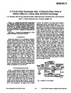
phase modulation of the pump becomes 20 ns and its spectral line spacing becomes 50 MHz. While this is larger than the Brillouin linewidth, the slow decay of the Lorentzian lineshape of SBS means there are still cross-interactions. We use a total temporal window of 0.26 µs, which corresponds to 13 × 20 ns of the phase modulation period and 20.8 fiber transit times. The Brillouin pump power was 200 W. Figure 2a shows Pareto optimization results. Each point corresponds to a specific optimized waveform, which fulfills the criterion that we found no other waveform which resulted in both a narrower linewidth and a lower Stokes power. For the same optimized modulation waveforms we calculated the corresponding Brillouin threshold power (Pth ), also shown in Fig. 2a. We define this as the power that leads to 1% Brillouin back-scattering. The threshold for an unmodulated laser is 41.8 W. In Fig. 2a, we also plot a line extrapolated from the unmodualted threshold according to, Pth =

kAef f ∆νp (1 + ) gB Lef f ΓB

(6)

The dependence of the SBS threshold on the linewidth is sometimes approximated by this equation [23], which can be viewed as an ideal upper limit on the threshold. This line is drawn in Fig. 2a along with the threshold values. The acoustic noise that seeds SBS was kept constant for every run in the optimization. This removes random fluctuations between runs, which otherwise can create problems for the optimization. Although the optimized modulation formats work well with that particular noise seeding, it is possible that it would be far worse with another random noise seeding. To assess this, we used the same modulation formats with fifty different cases of random noise seeding for seven optimized formats and calculated the resulting Brillouin threshold. Figure 2b shows the result. We see a maximum of 7% variation in Pth with random seeding. The fact that our optimization is over several periods, each with different random noise seeding, reduces the scope for the waveform to be exceptionally well suited to a specific pattern of the random noise, and less well suited to others. Like other approach to nonlinear optimization, the Paretooptimization of phase samples is not guaranteed to find the best solutions. To investigate this we select some of the modulation formats in Fig. 2a and add random values within a certain range to the corresponding phase samples. We then plot the resulting threshold and RMS linewidth on top of the data from Fig. 2a. Figure 3 shows the results. For most points, it is not possible to significantly improve the threshold without increasing the linewidth. This means that the Paretooptimization worked well. However, at fixed linewidth of 672 MHz in Fig. 3b we find that better optimized results can lead up to 10% enhanced threshold. We next exemplify the Pareto optimization results for two linewidths from Fig. 2. Figure 4a shows the optimized sampled phase points and the resulting continuous modulation waveform we calculated for 10 phase samples for an RMS linewidth of 676.9 MHz. The phase occasionally stretches beyond the

This work is licensed under a Creative Commons Attribution 3.0 License. For more information, see http://creativecommons.org/licenses/by/3.0/.

This article has been accepted for publication in a future issue of this journal, but has not been fully edited. Content may change prior to final publication. Citation information: DOI 10.1109/JSTQE.2017.2753041, IEEE Journal of Selected Topics in Quantum Electronics JOURNAL OF LATEX CLASS FILES, VOL. 6, NO. 1, JANUARY 2007

Fig. 2. (a) Pareto multi-objective optimization with 10 phase sample points of Stokes power vs. ∆νp calculated according to Eq. 5 on the right axis and plot of corresponding Brillouin threshold power calculated at 1% back-scatter on the left axis along with theoretical extrapolations according to Eq. (6) and (b) Brillouin threshold power for fifty different cases of noise seeding for seven modulation formats of Fig. 2a.

range of −π to π radians. This is because even though the sampled phase points are constrained within the (−π, +π) range, the continuous reconstructed signal can go beyond the range of the samples. Figure 4b shows the resulting optical power spectrum of the Brillouin pump (shifted to the baseband) along with the Brillouin Stokes spectrum in Fig. 4c. Note that the FWHM linewidth of the pump becomes 1.4 GHz, which is larger than the RMS linewidth by a factor of 2.1. Fig. 4 d-f repeat the graphs of Fig. 4 a-c, but for a linewidth of 197.8 MHz. In this case, the FWHM linewidth becomes 340 MHz, although this value depends significantly on whether certain spectral lines are slightly larger or slightly smaller than 50% of the peak line. Note also that even though the input pump spectra consist of discrete lines, the Stokes spectra are continuous (the spectral sampling of 3.85 MHz is only an artefact of our numerical grid, and is small compared to the Brillouin linewidth as well

5

Fig. 3. (a) Effect on the threshold values and RMS linewidth when 50 different set of random changes within a range of ±0.1 radians are added to each of 5 different optimized phase samples of Fig. 2a, (b) same as (a) with error range of ±0.5 radians.

as the 50 MHz spacing of the pump). Larger phase modulation amplitude increases the Brillouin threshold as well as the linewidth. Therefore, it is not obvious what effect a larger allowed phase amplitude will have on the Pareto front. Since it relaxes the constraints, some improvement is possible, but this may be small. Fig. 5a compares the results obtained with permissible phase modulation amplitudes of ±π and ±2π. The theoretical line extrapolation according to Eq. 6 is also shown for comparison in Fig. 5a. With ±2π allowable phase amplitude we see a 13.4 dB increase in the highest SBS threshold power with 1.3 GHz linewidth. It is interesting to note that this is getting close to the threshold for stimulated Raman scattering, which with a Raman gain coefficient of 40 fm/W becomes ∼1 kW for 1% Stokes power. This suggests that with optimization beyond this level of linewidth broadening, SBS is no longer the primary nonlinearity. The increase in threshold can also be compared to the 11.3 dB increase obtained with 672.5 MHz linewidth for ±π phase amplitude. However, larger maximum modulation amplitude

This work is licensed under a Creative Commons Attribution 3.0 License. For more information, see http://creativecommons.org/licenses/by/3.0/.

This article has been accepted for publication in a future issue of this journal, but has not been fully edited. Content may change prior to final publication. Citation information: DOI 10.1109/JSTQE.2017.2753041, IEEE Journal of Selected Topics in Quantum Electronics JOURNAL OF LATEX CLASS FILES, VOL. 6, NO. 1, JANUARY 2007

6

Fig. 4. (a) Phase modulation signal generated with 10 optimized phase samples for a pump linewidth of 676.9 MHz. (b) Corresponding Brillouin pump spectrum as launched into the fiber, (c) Brillouin Stokes spectrum calculated at the pump input end of the fiber. (d) Phase modulation signal generated with 10 optimized phase samples for a pump linewidth of 197.8 MHz. (e) Corresponding Brillouin pump spectrum and (f) Corresponding Brillouin Stokes spectrum.

does not lead to any clear increase in the SBS threshold at a given linewidth. In some cases, it even decreases. We attribute this to imperfect optimization. Presumably, the higher the range of allowed phase values for optimization, the higher is the probability of shortfalls in the calculations of the Pareto front. Although we have not made any direct attempts to assess how well the Pareto optimization and subsequent calculation of the threshold works, this and other graphs suggest that threshold improvements of up to 15% may be possible in some cases with more thorough optimization. Although this is significant, the availability of nearby data points makes it possible to identify points that seem less reliable and thus asses a curve on the whole with adequate confidence. The sampling frequency of the modulation signal is also an important factor. The considerations are similar as for the modulation amplitude. Fig. 5b compares the results of the Pareto optimization for sampling frequencies of 5 GHz (as in Fig. 2) and 2.5 GHz, wherein we optimized 10 and 5 phase samples (to keep the period the same), respectively. As for the case of an increase in the maximum amplitude, an increase in the modulation frequency increases the attainable threshold by increasing the attainable linewidth. However for similar linewidths the difference in threshold is small and may well

Fig. 5. (a) Plot of Brillouin threshold power vs. RMS linewidth for two different ranges of the phase modulation amplitudes where the 10 phase samples are constrained within ±π in one case and ±2π in another case for 2.5 m fiber length. (b) Plot of Brillouin threshold power vs. RMS linewidth for two different sampling frequencies of 5 GHz and 2.5 GHz for the same period (20 ns) and fiber length (2.5 m).

be caused by imperfect optimization. Next, to investigate the influence of the fiber length, we optimized 10 phase samples for 1 m, 1.5 m, 2.5 m, and 5 m fiber lengths with phase samples limited to ±π and with 20 ns period (spectral line spacing 50 MHz). The fiber transit time varies between 5 and 25 ns in these simulations, and the time window is 500 µs in order to reach 20 transit times also for the 5 m fiber. The corresponding Brillouin threshold power vs. linewidth characteristics are plotted in Fig. 6a. For small linewidths, Pth is largely inversely proportional to the fiber length, and the difference between 1 m and 5 m becomes 6.1 dB. This is close to the 7-dB suggested by the length ratio. For larger linewidths the difference becomes smaller than 6.1 dB, down to only 4.2 dB for 500 MHz. Fig. 6b plots Pth × L values against the ∆νp . We see that longer fibers show higher Pth × L values than shorter fibers. We believe that the reason

This work is licensed under a Creative Commons Attribution 3.0 License. For more information, see http://creativecommons.org/licenses/by/3.0/.

This article has been accepted for publication in a future issue of this journal, but has not been fully edited. Content may change prior to final publication. Citation information: DOI 10.1109/JSTQE.2017.2753041, IEEE Journal of Selected Topics in Quantum Electronics JOURNAL OF LATEX CLASS FILES, VOL. 6, NO. 1, JANUARY 2007

7

are therefore 210, 260, 280, and 320 ns.

Fig. 6. (a) Plot of SBS threshold power vs. RMS linewidth for four different fiber lengths of 1 m, 1.5 m, 2.5 m and 5m calculated with Pareto optimization of 10 phase samples and modulation depth of ±π and (b) plot of Pth × L values vs. linewidth for fiber lengths of 1 m, 1.5 m, 2.5 m and 5 m showing enhanced values of the product of SBS threshold and length for longer fibers.

is that the shorter fibers are too short for the phase relations between the spectral components of the interacting waves to be averaged as they propagate down the fiber. Thus, the phase relations are sometimes favorable for SBS. This lowers the threshold values due to additive cross-interactions. A similar behavior was observed in simulations by Zeringue et al. [19] and it was suggested that they had experimental data which was in agreement. The period of the phase modulation signal (T ) decides the spectral spacing of the frequency components, which is also a primary parameter of interest. Next we compare modulation periods ranging from 80 ns (12.5 MHz spectral spacing) to 10 ns (100 MHz spectral spacing) for a fiber length of 2.5 m. The sample frequency is kept at 5 GHz in all these cases. Hence, for 10 ns period we optimize 5 phase samples whereas for 80 ns period we optimize 40 phase samples. We keep the total temporal range to at least 20 transit times in all cases. The corresponding trace lengths for 10, 20, 40 and 80 ns periods

Fig. 7. (a) SBS threshold power against linewidth for different modulation periods, T = 10, 20, 40 and 80 ns with corresponding spectral spacing of 100 MHz, 50 MHz, 25 MHz and 12.5 MHz and (b) plot showing the threshold power against the linewidth divided by spectral line spacing approximating the number of lines within the RMS linewidth.

Figure 7a shows the results, i.e., Pth vs. ∆νp . The longest period of 80 ns performs better than the shorter modulation periods with larger spectral spacing. Figure 7b plots the SBS threshold against the RMS linewidth divided by the spectral line spacing. This is a measure of the number of spectral lines within the RMS linewidth. For the same number of spectral lines, a larger line-spacing gives a higher threshold power than a smaller spacing does. This is expected, because of the smaller overlap between the gain spectra of adjacent lines and the concomitant reduction of cross-interactions. Figure 8a shows how the (threshold×length) product depends on the line-spacing of the pump spectrum for RMS linewidths of 525 MHz for two fiber lengths, 1 and 2.5 m. The data for the fiber length of 2.5 m is extracted from Fig. 7a. According to basic theory, this product should be the same for both fiber lengths (at least for an unmodulated case), but it is significantly different for smaller line-spacings. However

This work is licensed under a Creative Commons Attribution 3.0 License. For more information, see http://creativecommons.org/licenses/by/3.0/.

This article has been accepted for publication in a future issue of this journal, but has not been fully edited. Content may change prior to final publication. Citation information: DOI 10.1109/JSTQE.2017.2753041, IEEE Journal of Selected Topics in Quantum Electronics JOURNAL OF LATEX CLASS FILES, VOL. 6, NO. 1, JANUARY 2007

8

the difference decreases for larger line spacings, as the crossinteractions become less important. Furthermore, the product improves for smaller line-spacings, i.e. for longer periods. It is actually clear that a longer period must be at least as good as a shorter one, if the sample rate is the same, at least if the longer period is an integer multiple of the shorter one. The reason is that the longer period can then exactly reproduce any waveform of the shorter period, so the longer period cannot be worse if the optimization works well. It is still theoretically possible that the optimum waveform of a, say, 80 ns waveform is (nearly) the same as four cascaded 20 ns waveforms. In this case, the actual line-spacing becomes 50 MHz (inverse of 20 ns rather than of 80 ns), with intermediate lines (nearly) void of power. To investigate this possibility, Fig. 8b-e plots the input spectra of the phase-modulated pump corresponding to the points in Fig. 7a, for the 2.5 m fiber. The spectral filling of the optimized points does increase for longer periods, and we conclude that with the optimized waveforms, the benefits of the increased spectral filling outweigh the disadvantages of the cross-interactions. It is interesting to compare the improvements in threshold we achieve to those of other approaches. Alternative phase modulation formats used for SBS suppression employ white noise source (WNS) [16], multi-frequency sine-waves [9] and pseudo-random binary sequences (PRBS) [24]. Here, modulation with multi-frequency sine-waves is similar to modulation with an AWG, and can be identical if the sine-waves are multiples of a common base frequency and have controlled phases. If not, we expect that multi-frequency sinewave modulation is worse, due to the uneven line-spacing, and/or lack of phase control. For noise modulation, and this in a typical experimental setup, random white noise is filtered through a low pass filter, amplified in an RF amplifier, and used to drive the electrooptic phase modulator [16],[25]. We next compare the increase in SBS threshold resulting from phase modulation with WNS with the Pareto-optimized results of Fig. 2, for a fiber length of 2.5 m. To simulate SBS suppression with WNS modulation, we generate WNS with a sampling frequency of 5 GHz. We use 130 noise samples at 2 ns sample period to reconstruct the noise modulation signal yielding the same temporal range of 0.26 µs as used for Fig. 2. The amplitude distribution of the noise samples depends on the details of the noise generator and any RF amplifier that is used. Here we assume that they result in phase samples that are uniformly distributed in the interval (−π, +π), when used to drive the phase modulator. The interval can be controlled by the settings of the RF amplifier. This noise modulation signal is used to drive the phase modulator. We determine the values of Pth and the optical RMS-linewidth ∆νp for these 130 samples, in the same way as we did for the optimized modulation waveforms. We perform this simulation for 1000 different random noise modulation waveforms, which, if we were to combine them, would add up to a total duration of 0.26 ms. Since the waveforms are random we get different results for each trial. Figure 9 shows a scatter-plot of the resulting data pairs. The

Fig. 8. (a) Plot of Pth × L against the spectral spacing at a linewidth of 525 MHz for fiber lengths of 2.5 m and 1 m and (b)-(e) pump power spectra for different spectral spacing of 12.5, 25, 50 and 100 MHz for the same RMS linewidth of 525 MHz in case of 2.5 m fiber legnth.

This work is licensed under a Creative Commons Attribution 3.0 License. For more information, see http://creativecommons.org/licenses/by/3.0/.

This article has been accepted for publication in a future issue of this journal, but has not been fully edited. Content may change prior to final publication. Citation information: DOI 10.1109/JSTQE.2017.2753041, IEEE Journal of Selected Topics in Quantum Electronics JOURNAL OF LATEX CLASS FILES, VOL. 6, NO. 1, JANUARY 2007

9

average ∆νp for WNS modulation evaluates to 511.4 MHz and the average Pth evaluates to 257.9 W. For comparison, we also re-plot the optimized Pth vs. ∆νp characteristics from Fig. 2b.

Fig. 10. (a) Plot of number of counts in 100 bins from 0 to 570 W against the Brillouin threshold power for 1000 trials with WNS modulation for fiber length of 2.5 m. (b) similar plot of number of counts in 100 bins from 0 to 676.9 MHz against the ∆νp .

Fig. 9. Scatter plot of Pth vs. ∆νp for 1000 trials of WNS modulation for fiber length of 2.5 m along with the results of the optimized formats and theoretical line included for comparison.

Unsurprisingly, the optimized waveforms are far better than the random ones in several ways. First of all, no random waveform qualifies for inclusion on the Pareto front (as reevaluated from Stokes power to threshold power). This means that for each random waveform, there is an optimized waveform which is better in both threshold power and linewidth. Furthermore, at the average linewidth of 511.4 MHz for the random waveforms, the optimized threshold becomes 434.8 W. This is 1.6 times higher than the average threshold power for the random waveforms of 257.9 W, and 4.1 times higher than the minimum threshold power for the random waveforms of 107.2 W (within a total time of 0.26 ms). In order to avoid potentially disastrous SBS-spikes with random modulation, the power should be kept below this minimum threshold power. However, with optimization, the same threshold power is reached already with a linewidth of 100.1 MHz. Although points outlying in linewidth are typically a smaller concern than those outlying in threshold power, we also note that the random modulation occasionally leads to linewidths of 696.9 MHz, which is 6.9 times larger than 100.1 MHz. Fig. 10 shows distribution functions of Pth and ∆νp , each divided into 100 bins, for the 1000 random modulations. These plots show a standard deviation of 105.8 W for Pth and 112.2 MHz for the linewidth. As it comes to the variation in linewidth, there is 8% probability for the linewidth (as evaluated in 0.26 s) to exceed 600 MHz and 22.8% probability to exceed 500 MHz. Note also that the variations are much larger than those resulting from the random acoustic noise variation in Fig. 2c. These variations are crucial when we want to operate the laser with desired specifications in applications like coherent beam combining. In this regard the optimized phase modulation formats seem far superior to noise modulation. Pseudo-random binary sequences (PRBS) with π phase

shifts have also been studied extensively for SBS suppression [24]. The bit sequences are chosen randomly which is unlikely to be the best solution. It is however quite possible that through optimization, PRBS can yield comparable performance, but this is beyond the scope of this work. PRBS modulation is attractive in that suitable drivers are cheaper than an AWG for the same sample frequency, although it is likely that a higher PRBS sampling frequency would be required to compensate for the higher freedom of an AWG. Having said that, the 500 MHz sampling frequency we typically used is far from stateof-the art, and even AWGs would be relatively inexpensive. Even if we disregard the possibility of alternative modulation approaches, the parameter space is very large. We have only investigated a small sample, dictated in part by limits in computers and software we have used. For example, higher sample frequencies and longer modulation periods would be interesting to investigate, as well as if the curves in Fig. 5c would converge for longer fibers, as we believe they should. While RMS linewidth is a convenient measure, other can be more appropriate, for example beam-combination efficiency or “power-in-bucket” (e.g., power within a certain linewidth). A problem with these measures is that they introduce additional parameters of interest. In case of power-in-bucket, the power and the spectral width of the “bucket” are both of interest. Combined with the Brillouin threshold power, this then creates a three-dimensional Pareto front. Although more dimensions are more difficult or impossible to illustrate, the increase in the computational burden can be more modest, which is a key attraction of Pareto optimization. Most important for run-times are the number of phase-samples to be optimized and the numerical solution of the Brillouin equations. Powerin-bucket Pareto optimization calls for lengthier processing of each solution of the Brillouin equations, but it does not necessarily require us to increase the number of times we solve the equations. Therefore, the increase in run-times can be modest. Finally, a major point of the work presented here is that we use a passive fiber (e.g. a delivery fiber) to find optimized formats. We expect that fiber amplifiers will lead to significant differences in the optimized waveforms.

This work is licensed under a Creative Commons Attribution 3.0 License. For more information, see http://creativecommons.org/licenses/by/3.0/.

This article has been accepted for publication in a future issue of this journal, but has not been fully edited. Content may change prior to final publication. Citation information: DOI 10.1109/JSTQE.2017.2753041, IEEE Journal of Selected Topics in Quantum Electronics JOURNAL OF LATEX CLASS FILES, VOL. 6, NO. 1, JANUARY 2007

V.

C ONCLUSION

We theoretically investigated suppression of SBS in singlemode optical fibers through periodic phase-modulation. This leads to a broadened optical spectrum with discrete lines. The spectral lines are sufficiently close together for coherent crossinteractions between the lines to be important. Therefore, their relative phase matters, and because the fibers are short (1-5 m), the phase relations are not fully averaged along the fiber. We use a time-domain finite difference solver to account for these factors in the SBS process. More broadening leads to better suppression. We used multi-parameter Pareto optimization to find modulations that represent the best trade-off between SBS suppression and the optical linewidth, as measured by its RMS value. Our modeling assumes an arbitrary waveform generator connected to a phase modulator, and the optimization finds sample values for the phase that maximizes the suppression. We discussed the influence of the maximum phase modulation depth and sampling frequency, fiber length, spectral-line spacing and random noise seeding. Although shorter fibers have a higher threshold, the increase is smaller than the often-assumed inverse dependence on length. Although larger maximum modulation depth and sampling frequency allow for higher SBS threshold, this is only insofar as the linewidth is increased. On the other hand, with proper optimization, a closer line spacing does improve the SBS suppression for a given linewidth. We also find that the optimized formats are superior in terms of SBS threshold as well as in terms of linewidth control, compared to random modulation. This work does not take into account the mechanisms of an optical fiber amplifier. This may be studied as a future work along with exploring cost function formulation that lead to better optimized results. R EFERENCES [1] R. G. Smith, “Optical power handling capacity of low loss optical fibers as determined by stimulated Raman and Brillouin scattering,” Appl. Opt., vol. 11, no. 11, pp. 2489–2494, Nov 1972. [2] A. Liem, J. Limpert, H. Zellmer, and A. T¨unnermann, “100-w singlefrequency master-oscillator fiber power amplifier,” Opt. Lett., vol. 28, no. 17, pp. 1537–1539, Sep 2003. [3] “Single-frequency, single-mode, plane-polarized ytterbium-doped fiber master oscillator power amplifier source with 264 W of output power.” Optics letters, vol. 30, no. 5, pp. 459–461, 2005. [4] S. Yoo, C. a. Codemard, Y. Jeong, J. K. Sahu, and J. Nilsson, “Analysis and optimization of acoustic speed profiles with large transverse variations for mitigation of stimulated Brillouin scattering in optical fibers.” Applied optics, vol. 49, no. 8, pp. 1388–99, mar 2010. [5] F. H. Mountfort, S. Yoo, A. J. Boyland, A. S. Webb, J. Nilsson, and J. K. Sahu, “Temperature effect on the Brillouin gain spectra of highly doped aluminosilicate fibers,” in 2011 Conference on Lasers and ElectroOptics Europe and 12th European Quantum Electronics Conference, CLEO EUROPE/EQEC 2011, 2011. [6] Y. Jeong, J. Nilsson, J. K. Sahu, D. N. Payne, R. Horley, L. M. B. Hickey, and P. W. Turner, “Power scaling of single-frequency ytterbiumdoped fiber master-oscillator power-amplifier sources up to 500 w,” IEEE Journal of Selected Topics in Quantum Electronics, vol. 13, no. 3, pp. 546–551, May 2007.

10

[7] Y. Jeong, J. K. Sahu, D. B. S. Soh, C. a. Codemard, and J. Nilsson, “High-power tunable single-frequency single-mode erbium:ytterbium codoped large-core fiber master-oscillator power amplifier source.” Optics letters, vol. 30, no. 22, pp. 2997–2999, 2005. [8] A. V. Harish and J. Nilsson, “Optimization of phase modulation with arbitrary waveform generators for optical spectral control and suppression of stimulated scattering,” Opt. Express, vol. 23, no. 6, pp. 6988–6999, Mar 2015. [9] S. Korotky, P. Hansen, L. Eskildsen, and J. Veselka, “Efficient phase modulation scheme for suppressing Stimulated Brillouin scattering,” in Tech. Dig. Int. Conf. Integrated Optics and Optical Fiber Comm.vol 1, 1995, pp. 110–111. [10] R. T. Logan and R. D. Li, “Method and apparatus for optimizing sbs performance in an optical communication system using at least two phase modulation tones,” U.S. patent 6,282,003, Aug 2001. [11] S. K. Korotky, “Multifrequency lightwave source using phase modulation for suppressing stimulated brillouin scattering in optical fibers,” U.S. patent 5,566,381, Oct 1996. [12] T. Torounidis, P. A. Andrekson, and B. E. Olsson, “Fiber-optical parametric amplifier with 70-db gain,” IEEE Photonics Technology Letters, vol. 18, no. 10, pp. 1194–1196, May 2006. [13] S. Hocquet, D. Penninckx, J.-F. Gleyze, C. Gou´edard, and Y. Jaou¨en, “Nonsinusoidal phase modulations for high-power laser performance control: stimulated Brillouin scattering and FM-to-AM conversion,” Applied Optics, vol. 49, no. 7, p. 1104, 2010. [14] C. Zeringue, I. Dajani, S. Naderi, G. T. Moore, and C. Robin, “A theoretical study of transient stimulated Brillouin scattering in optical fibers seeded with phase-modulated light,” Opt. Express, vol. 20, no. 19, pp. 21 196–21 213, Sep 2012. [15] A. Flores, C. Lu, C. Robin, S. Naderi, C. Vergien, and I. Dajani, “Experimental and theoretical studies of phase modulation in yb-doped fiber amplifiers,” pp. 83 811B–83 811B–8, 2012. [16] A. Mussot, M. Le Parquier, and P. Szriftgiser, “Thermal noise for SBS suppression in fiber optical parametric amplifiers,” Optics Communications, vol. 283, no. 12, pp. 2607–2610, jun 2010. [17] J. B. Coles, B. P.-P. Kuo, N. Alic, S. Moro, C.-S. Bres, J. M. Chavez Boggio, P. a. Andrekson, M. Karlsson, and S. Radic, “Bandwidthefficient phase modulation techniques for stimulated Brillouin scattering suppression in fiber optic parametric amplifiers.” Optics express, vol. 18, no. 17, pp. 18 138–18 150, 2010. [18] R. W. Boyd, K. Rza¸ewski, and P. Narum, “Noise initiation of stimulated Brillouin scattering,” Phys. Rev. A, vol. 42, pp. 5514–5521, Nov 1990. [19] C. Zeringue, I. Dajani, S. Naderi, G. T. Moore, and C. Robin, “A theoretical study of transient stimulated Brillouin scattering in optical fibers seeded with phase-modulated light.” Optics express, vol. 20, no. 19, pp. 21 196–213, 2012. [20] A. V. Harish and J. Nilsson, “Arbitrary phase modulation for optical spectral control and suppression of stimulated Brillouin scattering,” pp. 94 660M–94 660M–8, 2015. [21] R. Marler and J. Arora, “Survey of multi-objective optimization methods for engineering,” Structural and Multidisciplinary Optimization, vol. 26, no. 6, pp. 369–395, 2004. [22] “Multiobjective optimization: Minimize multiple objective functions subject to constraints,” Mathworks, 2015. [23] D. A. Fishman and J. A. Nagel, “Degradations due to stimulated brillouin scattering in multigigabit intensity-modulated fiber-optic systems,” Journal of Lightwave Technology, vol. 11, no. 11, pp. 1721–1728, Nov 1993. [24] A. Flores, C. Robin, A. Lanari, and I. Dajani, “Pseudo-random binary sequence phase modulation for narrow linewidth, kilowatt, monolithic fiber amplifiers,” Opt. Express, vol. 22, no. 15, pp. 17 735–17 744, Jul 2014. [25] B. Anderson, A. Flores, R. Holten, and I. Dajani, “Comparison of phase modulation schemes for coherently combined fiber amplifiers,” Opt. Express, vol. 23, no. 21, pp. 27 046–27 060, Oct 2015.

This work is licensed under a Creative Commons Attribution 3.0 License. For more information, see http://creativecommons.org/licenses/by/3.0/.

This article has been accepted for publication in a future issue of this journal, but has not been fully edited. Content may change prior to final publication. Citation information: DOI 10.1109/JSTQE.2017.2753041, IEEE Journal of Selected Topics in Quantum Electronics JOURNAL OF LATEX CLASS FILES, VOL. 6, NO. 1, JANUARY 2007

A.V. Harish is a Ph.D. student at the ORC, University of Southampton, UK, and member of the High Power Fiber Lasers research group. He obtained his master of Science degree from Indian Institute of Technology Madras (IIT-M), Chennai, India. He has worked on optical fiber amplifiers, non-linear fiber optics at ORC and non-destructive testing with optical fiber sensors at IIT-M. He has published some 15 scientific articles. He is an active member of the Optical society (OPSoc) at University of Southampton. He is a student member of the OSA, IEEE Photonics society and the SPIE. His current research interests include suppression of stimulated Brillouin scattering in high power optical fiber amplifiers, advanced optical modulation and non-destructive testing of structures using fiber Bragg gratings.

Johan Nilsson is a Professor at the ORC, University of Southampton, UK, and head of the High Power Fiber Lasers research group. In 1994, he received a doctorate in Engineering Science from the Royal Institute of Technology, Stockholm, Sweden, for research on optical amplification. Since then, he has worked on optical amplifiers and amplification in lightwave systems, optical communications, and guided-wave lasers, first at Samsung Electronics and later at ORC. His research has covered system, fabrication, and materials aspects, and in particular device aspects of high power fiber lasers and erbium-doped fiber amplifiers. He has published some 400 scientific articles. He is a fellow of the OSA and the SPIE, and a consultant to, and co-founder of, SPI Lasers. He is a member of the advisory board of the Journal of the Optical Society of Korea and was guest editor of two issues on high-power fiber lasers in IEEE Journal of Selected Topics in Quantum Electronics in 2009. He is a former chair of the Laser Science and Engineering technical group in OSAs Science and Engineering Council and is currently program chair for the EuroPhoton and Advanced Solid State Lasers conferences.

This work is licensed under a Creative Commons Attribution 3.0 License. For more information, see http://creativecommons.org/licenses/by/3.0/.

11