Optimization of Self-Organizing Maps Ensemble in Prediction Elie Prudhomme Abstract— The knowledge discovery process encounters the difficulties to analyze large amount of data. Indeed, some theoretical problems related to high dimensional spaces then appear and degrade the predictive capacity of algorithms. In this paper, we propose a new methodology to get a better representation and prediction of huge datasets. For that purpose, an ensemble approach is used to overcome problems related to high dimensional spaces. Self-Organized Map, which allows both a fast learning and a navigation through the data is used like base classifiers to learn several feature subspaces. A genetic algorithm optimizes diversity of the ensemble thanks to an adapted error measure. The experimentations show that this measure helps to construct a concise ensemble keeping representation capabilities. Furthermore, this approach is competitive in prediction with Boosting and Random Forests.
I. M OTIVATIONS Because storage was no more subjected to important constraints of cost, the information systems collect an increasing quantity of data. At the same time, objects of interest become more complex. For example, let’s cite collections of images, texts or DNA chips. This conjunction jointly increases the number of examples and features describing such databases. Learning algorithms have to take into account this evolution. Indeed, the traditional tools of machine learning are not always adapted to this new volume of data (Verleysen, 2003) and may encounter problems at all the stages of the analysis. The first challenge relates to the time needed by the algorithm to build its predictive model and is directly linked to the quantity of data to analyse. Consequently, methods without linear complexity according to examples and features would not ensure scalability with bulky data. To be used, they need heuristics or sampling strategies which could degrade the learning result. Furthermore, a growing number of features leads to theoretical problems for learning algorithms. First, the number of points needed to describe space grows exponentially with its dimensionality (curse of dimensionality, Bellmann (1975)). The learning thus loses in precision in high dimensional spaces. Then, distances between points tend to be constant at space infinity (concentration of measures, Demartines (1994)). These phenomenons have consequences that render mandatory the adaptation of learning algorithms (Verleysen et al., 2003). Moreover, concentration of measures compromises navigation through examples. Yet, this navigation is useful during the prediction stage. It allows to show to the user Elie Prudhomme and St´ephane Lallich are with the ERIC Laboratory, University of Lyon, Bron:France (email:
[email protected] and
[email protected]).
St´ephane Lallich examples similar to his request and already classified in the system. These examples help the user to confirm if the prediction model is correct and eventually to adjust it. Finally, this kind of strategy adds an explicative dimension to the model. A good learning process of huge datasets must allow both navigation and visualisation, adapting its algorithm to the specific problem of high dimensional spaces. The novelty of this paper is to present an ensemble of Self-Organized Maps (SOM) as an answer for these problems. Ensembles (see Valentini and Masulli (2002) for a review) are sets of weak learning machines whose decisions are combined to improve performance of overall system. They bring interesting solutions to problem of high dimensional spaces by dividing the feature space into smaller sizes subspaces each of them learned by different classifiers. The classifiers we used here are based on Self-Organizing Maps. These later confer a fast learning as well as a representation of the data. The rest of this paper is organized as follows. The next section presents ensembles (Sect. II) with a focus on the diversity notion and theoretical results obtained on ensemble error. These results allow us to optimize size and error rate of a maps ensemble with a genetic algorithm (Sect. III). At last, the validation by experimentations of this strategy on high dimensional datasets is presented in Sect. IV. II. E NSEMBLE APPROACH A. Introduction Ensembles combine several classifiers to improve the learning. It includes bagging (Breiman, 1996), boosting (Freund, 1990) or random forest (Breiman, 2001). This implies a three-step learning. First, the information (carried by examples, features or classes) is shared out between several classifiers. Then, this information is learned by each one. Finally, their prediction is combined to get the class of a new example. Such approach has been applied to a wide range of real problems with theoretical and empirical evidences of its effectiveness. For example, bagging (Boostrap AGGregatING) builds L classifiers by making bootstrap replicates of the learning set (Breiman, 1996). In this way, bagging reduces error variance, mainly due to the learning set. In bagging, samples are drawn with replacement using an uniform probability distribution, whereas in boosting methods (Freund, 1990) weighted samples are drawn from training data. That technique places the highest weight on examples misclassified by the last base classifiers. Thus, boosting enlarges margins of the training set and then reduces the generalization error. Those two methods sample the training set to learn different classifiers however this is not
the only strategy to build ensembles. For example, in mixture of experts, each classifier are competing each others to learn an example (Jacobs et al., 1991). Or, when data are stemming from several sensors, each classifier learns data belonging to a specific one (Duin and Tax (2000)). A more complete description of ensembles could be found in Valentini and Masulli (2002). B. Diversity and Error Measures One of the major reasons of the ensembles success is summarized by diversity concept (Brown et al. (2005) for a review). Although there is no formal definition, diversity is the capability of different classifiers to make their mistakes on different examples. Indeed, the more the classifiers are mistaken on different examples of the training set, the more it is probable that a majority of them find the correct response for a specific example. That intuition on diversity was confirmed by several theoretical results, described in the next paragraph. The first work were conducted on regression ensembles (Geman et al., 1992; Krogh and Vedelsby, 1995). They demonstrate that error from one ensemble comprise two terms, one being the mean error of classifiers and the other corresponding to their variability. This second term is composed of variance as well as covariance (thus diversity) from the classifiers error. In a classification context, the problem is formulated differently by Tumer and Ghosh (1995). They are interested in a posteriori probabilities predicting each class, to show that the error from an ensemble is linked to the correlation between the errors of the classifiers. Recently, Zanda et al. (2007a) used this framework to express the added error of an ensemble in a classification context. They reduced Tumer and Gosh model to a regression problem. Therefore, they identified the differences between the true posterior probability of each class as target of regression given an example x (denoted dij = P (i|x) − P (j|x), where P (i|x) is the true posterior probability of class i) and as estimation of the differnce between the estimated posterior probability of each class given that example (f¯ij = f¯i (x) − f¯j (x), where f¯i (x) is the estimated posterior probability of class i). Once, reduced to a regression problem, they take advantage of previous work (Krogh and Vedelsby, 1995) and express the error added by an ensemble with: E
=
C X X
(f¯ij − dij )2
i=1 j>i
"
# M 1 X m 2 = (f − dij ) M m=1 ij i=1 j>i # " M C X X 1 X ¯ m 2 (fij − fij ) − M m=1 i=1 j>i C X X
¯−A . = E where M is the ensemble size ; C, the number of classes ; fim , the posterior probability for the mth classifier to predict m = fim − fjm . Similar to the regression model, class i and fij
¯ is that error could be broken into two terms. The first (E) the base classifiers mean error and the second (A) contains a measure of the diversity. By increasing diversity with a ¯ it becomes possible to reduce the ensemble error. constant E, III. M APS E NSEMBLES In case of high dimensional datasets, we propose to set up an ensemble of self-organized maps (SOM). After a brief presentation of SOM in supervised learning (Sect. III-A), we give details on the methodology used to build our ensemble (Sect. III-B). Finally, we consider two aggregation schemes of the base classifiers results (Sect. III-C). A. SOM in Supervised Learning SOM allows both a fast unsupervised learning of examples and their representation. Because of those properties (fast algorithm and topology preservation), they have been adapted to a supervised learning composed of two steps. At first, the class of examples is only used after a classical learning of SOM on features. Then during the second step, neurons take the class of the examples they represent. The reverse happens during prediction: the class of a new example is determined by the class of the neuron which best matches that example with the Kohonen-Opt function (Prudhomme and Lallich, 2005). It specifies the class of the empty neurons (which doesn’t match any example) or undeterminates (which match as much examples of different classes). Even if this method aims class prediction, it could easily be used to estimate the posterior probability of each class for a new example. This probability is computed as the proportion of examples corresponding to the class. In case of an empty neuron, probabilities of the nearest neighbor are used. B. Subspaces Selection by Genetic Algorithm As underlined in Sect. II-B, ensemble error depends on both mean error of its base classifiers and on diversity measure of these classifiers. To improve the ensemble performance, these two parts of the error must be optimized. However, an increase in the diversity leads often to decreasing the base classifiers performance. This trade-off could be solved by several strategies, the first one uses hazard. For example, random forests arbitrarily select subspace for each tree. Likewise, bagging randomly picks example to learn. It is also possible to use heuristics. In a previous work, we have managed diversity and mean error thanks to a feature clustering (Prudhomme and Lallich, 2008). Finally, this trade-off could be optimized through the ensemble error either during the learning (this is the case for Boosting or Negative Correlation (Brown, 2005; Zanda et al., 2007b)) or after, to select the best ensemble (Zhou et al., 2001; Oliveira et al., 2003). In this paper, we propose to exploit the work of Zanda et al. which expresses the ensemble error in classification. This measure is applied to the selection of the best ensemble. To overcome the shortcomings of high-dimensional spaces, we dispatch the learning on several maps, each one
learned from different feature subspaces. As different maps learn different groups of features, an important number of features are used, conversely to a feature selection during the preprocessing step. The advantage, as underlines Verleysen et al. (2003), is that the redundancy of information takes part in the noise reduction on each feature. Thus, for high dimensional data, ensemble can handle information in its globality while it circumvents problems arising from high dimensional space. That feature partitioning generates some diversity but do not guarantees an optimally distributed diversity between base classifiers of relatively good quality. To ensure this, we realized the optimization of E by a Genetic Algorithm (GA). The search space of this GA grows exponentially with the number of features. As we consider high dimensional space, we set up two heuristics in order to limit the GA √ search. First, we only take a look at subspace of size D0 = D features (where D is the number of features in the original set). This little size increases the probability of reaching diversity in the maps prediction while allowing subspaces with enough of features to learn maps of relatively good quality. Second, to control the maps number (ie the ensemble size), we choose to care about only k subspaces. These k subspaces are randomly generated before the beginning of the GA optimization. Thus, we address the problem of finding, given k maps learned on D0 features, the subset of maps which optimizes the E measure. This optimization is done by a genetic algorithm. Its fitness function is the E measure. Individuals handled by GA are binary vector of length k. Their ith byte encodes presence (1) or absence (0) of the ith map in the final ensemble. The optimization is realized by utilizing the standard genetic algorithm (Goldberg, 1989). A new population is selected from the original population by the roulette wheel mechanism: each individual is associated to a probability p, proportional to its fitness, and is then reproduced with that probability. Consequently, some individuals (the best ones) are then more likely reproduced and some others (the worst ones) rejected. Genetic operators (cross-over and mutation) are applied on that population. That process is reiterated until all objects have a fitness of 1 (convergence) or number of iteration reaches a certain threshold (see Fig. 1). For example, if D = 100 and k = 12, 12 maps are learned on subspace of size 10. Next, the GA search the more effective set of maps according to the E measure. The individuals the GA evaluates look like 1 0 0 1 1 0 1 1 0 0 0 1. This one symbolizes an ensemble composed of the 6 maps numbered 1, 4, 5, 7, 8, 12. To compute the fitness, a validation subset is randomly picked from the learning set. For these examples, the posteriori probability fi of each class i is estimated on each map. Afterward, f¯i , the mean of fi on the ensemble, f¯ij and finally E are computed. The fitness is the sum of E for all examples in the validation set.
Fig. 1.
The different steps to optimize an ensemble with a GA.
C. Aggregation At the end of learning, the individual with the highest fitness is selected to define base classifier to incorporate in the final ensemble. Prediction of new example is then realized by aggregating maps prediction. We studied two aggregation schemes. For Majority Vote (MV), the class attributed to a new example is the one predicted by a majority of maps. This method is fast and easy to use. Furthermore, it performs often as well as more complex methods (Duin and Tax, 2000). For Weighted Vote (WV), each map assesses, given a new example, the estimated posterior probability of each class. Those probabilities are then added up and the class with the highest score is assigned to the example. This method is more complex than MV although it is consistent with the error measure optimized by GA. D. Scalability The two heuristics on the search for the best set of subspaces limit considerably the computation. Thus, the number of learned maps √ and the subspace size are respectively narrow to k and D. These k maps are learned only one time before the GA optimization. The √ maps learning step has a complexity of O(k × w × n × D) where n is the number of example and w the number of neurons. The search of the best ensemble requires the computation of E for each individuals of the GA at each generation (where I is the number of individuals and G, the number of generation). This evaluation requires the prediction of the estimated posterior probability of each class on the different maps for the examples of the validation set denoted by n0 , n0 < n. Therefore, the computational complexity of the GA is O(I × G × n0 × c2 ) (where c is the number of class). IV. E XPERIMENTATIONS On the several datasets used, parameters of our approach did not change. The maps had a size of 20 × 20 with
rectangular lattice of the grid. Examples of the learning set were presented 17 times in the same order with a learning rate and a neighborhood kernel which decreased linearly. For the genetic algorithms, we used standard parameters. The population had 40 individuals of size k = 100 (which implies 100 maps) and we computed 1500 generations. For each one, the cross-over and mutation rate were respectively 0.8 and 0.05. We made the choice to keep these parameters during all the experimentation to evaluate the robustness of our approach. Moreover, a fine tuning of parameters could bias the comparison with other approaches. Finally, in all experiments, error rates presented in tables and figures are averaged over 5 5-cross validations.
in figure 2. It shows that the optimal number of maps ranges between 35 and 45 (for an error rate of 7.1) while using GA strategy, ensemble size goes down to 13 maps for an error rate of 5.3 (using a Weighted Vote). After 45 maps, error rate does not decrease more, certainly because the added maps are incapable of increasing the diversity and then to reduce the ensemble error. 0.12 0.11 0.1 E.R. 0.09
A. Preliminary Experimentations
0.08
In order to set up our methodology, preliminary experiments were done on Ionosphere dataset. It had 33 features, 351 examples and 2 classes. Maps used by ensemble are selected by the GA from 100 maps learned on random subspaces. Average error rate of those maps was 12.98 ± 0.006 whereas their aggregation has an error rate of 7.19. Difference between these two error rates (+5.79%) was only due to ensemble approach (aggregation of weak classifiers). The GA objective had two parts: decrease the error rate and the size of this ensemble. The results obtained by several maps ensemble (in terms of error rate (E.R.) and ensemble size (Size)) are exposed in Table I. These ensembles were set up either from 20 maps randomly choose (Rand.) or with a GA optimizing E with aggregation by Majority Vote (GAE + M V ), or with a GA optimizing E with aggregation by Weighted Vote (GAE + W V ), or with a GA optimizing the error rate with aggregation by Weighted Vote (GAER + W V ). Results first suggest that aggregation by Weighted Vote gives better results than Majority Vote. It can be explained by adequacy between fitness and Weighed Vote. Indeed, Weighted Vote and fitness use together posterior probabilities to assess maps prediction. Then, results show the effectiveness of the E optimization. This optimization generates a lower error rates than an equivalent number of randomly chosen maps or the error rate optimization. The E optimization also allows to control, through the diversity, the size of the final ensemble. Thus, ensemble optimized by E contains only 13 maps whereas those optimized by the error rate raise to 51 maps. Diversity is not only a way to decrease the ensemble size but also a way to ensure a better generalization. Measure used is thus competitive qualitatively and quantitatively.
0.07
TABLE I C OMPARAISON OF DIFFERENT M APS E NSEMBLE ON I ONOSPHERE E.R. Size
Rand. 7.6 15
GAE + MV 6.7 13
GAE + WV 5.3 13
GAER + WV 6.6 51
In a second experiment, we sought for the optimum size of an ensemble of randomly chosen maps. Error rates of such ensemble according to number of maps used are presented
0.06 10
20
30
40
50
60
Ensemble Size
Fig. 2.
Error Rate (E.R.) with ensemble size on Ionosphere dataset.
Finally, we compared our approach to a single map (Kohonen-Opt), boosting and random-forest (two common ensemble approaches) (Table II). On these ionosphere datasets, maps ensemble optimized by GAwas more powerful than boosting or random forests. TABLE II M ETHODS COMPARAISON ON I ONOSPHERE DATASET Maps Ensemble GAE + W V 5.3
KohonenOpt 11.4
Boosting ID3 8.5
Random Forest 6.0
Preliminary tests gave us several indications. First, as ensemble, our strategy ensures better prediction compared with single classifiers. More interesting, the used measure E decreases the error linked to an ensemble of randomly chosen maps. This measure also optimizes ensemble size by selecting the most diverse maps. For these reasons, measure E is better suited than error rate which not takes diversity into account. Lastly, Weighted Vote accesses maps prediction in the same way that fitness and thus improves prediction comparing to Majority Vote. B. Comparisons After these preliminary tests, we compared our approach to Boosting, Random Forest and ID3 on several datasets from UCI (Newman et al., 1998). For these algorithms, we used Tanagra’s implementation (Rakotomalala, 2005). Their characteristics in terms of number of features, classes and examples are presented in Table III. Error rates obtained are shown in Table IV (datasets are represented by their number in Table III). Results of our approach are always better than ID3 . For dataset (1), our approach is between Random Forests and
TABLE III 40
DATASETS Datasets (1) Wbdc (2) Ionosphre (3) Spambase (4) Optdigits (5) Multi-features (Profile) (6) Spectrometer lrs (7) Multi-features (Fourier)
Features 31 34 58 64 76 100 216
Classes 2 2 2 10 10 10 10
Examples 561 351 4601 5619 2000 531 2000
C OMPARISON BETWEEN METHODS DEPENDING ON ERROR RATES . Maps ensemble 3.6 5.3 7.8 5.3 20.5 12.3 4.22
ID3 7.72 10.1 10.0 12.5 33.3 16.5 26.3
Random Forest Boosting Maps Ensemble
30
× 2 3 ×
25
× 2
E.R 20 15
TABLE IV Datasets 1 2 3 4 5 6 7
2
35
Boosting 2.8 8.5 5.6 5.2 37.6 10.3 8.1
Rand. Forests 4.9 6.0 5.5 2.3 21.6 11.7 5.6
10 5
3 × 2
2 3 ×
2 3 ×
2 × 3
5
10
15
× 2 3
× 2 3
× 2 3
3
3
0 0
20 25 Noise rate
30
35
40
Fig. 3. Error Rate (E.R.) evolution with noise rate on label for random forests, boosting and maps ensemble on Spambase data.
Boosting and for datasets (2), (5) and (7), it is the most competitive. Dataset (5) is interesting because, on that dataset, boosting gives worst results than ID3 (several parameters have been tested). That occurs when boosting overfits data, generally when data are noisy. In this case, our approach still gives interesting results, better than those obtained by Random Forests. C. Noise Resistance We investigated further the noise resistance of our approach on the dataset Spambase. For this dataset, 60% of examples described text of spam. We generated 8 new datasets from the original one. For each, noise have been added to the label with probabilities varying from 5 to 40% (by step of 5%). For these new datasets, an example had two class labels: the true label and the noisy label. Each dataset had been learned either by a maps ensemble or by random forests or boosting with the noisy label as target. On the contrary, error rate was estimated on the capacity of these classifiers to predict the true label. Thus, we tested the capacity to predict the class label despite the noise. Results of this experimentation are reported in the figure 3. In this figure, each method responds differently when the noise increase. For the random forests, error rate in generalization increases exponentially with the noise (r2 (ln y, ln x) = 0.99). The boosting reaction is more complex. First, a small increase in noise (5%) implies a strong increase in error rate (×2). This noise effect remains stable until 15%. Next, error rate grows exponentially, in the same way that the random forests. Finally, when noise rate reaches 40%, the boosting predict the majority label (Spam) for each new examples. As this label characterize 60% of the examples, the resulting error rate is 40%. Finally, for the maps ensemble, 30% of noise implies an increase of only 5, 2% in error rates. This strategy is the most robust to class noise and, on this dataset, it becomes the most performant for 15% of class noise.
The learning strategy of each method can explain these results. Boosting focus its learning on the most difficult examples during iterations. Yet, the noisy data are difficult to learn and boosting these data increases their importance on the prediction and decreases the performance. In the random forests algorithm, class label are used during the learning (in the choice of the features and discretization points used for learn each tree) and to predict the class of a new example (which is function of learning examples class already present in the tree nodes). The label noise then affects random forests at two stages. On the contrary, maps ensemble does not use the label to build its model (maps are unsupervised) but only to predict the class of a new example (which is function of learning examples class already present in the map neurons). Maps ensembles are then robust to noise because they base their learning on the data representation. V. C ONCLUSION This paper explains the advantages of maps ensemble in high dimensional space. By splitting features space to learn several classifiers, ensemble sidesteps high dimensional curses. In those conditions, maps ensemble enhances prediction of a single SOM. Features space splitting is conducted by the quality measure E optimized by a GA. This measure ensures the ensemble uses diverse and good classifiers. Thus, ensemble is both concise and competitive. Inversely, Random Forests randomly split features space and produce more base classifiers than our approach. Finally, this paper shows the relevance of SOM in ensemble approach. They represent data to predict new example. This representation helps to ensure data quality. Thanks to this, SOM are robust to process noisy data. Association between SOM and ensembles seems to be interesting to handle large datasets. Indeed, in addition to their low complexity, SOM are able to represent data spa-
tially, in opposition to boosting and random forest. Moreover using GA to optimize diversity limits the number of maps to represent data. User has thus a concise maps ensemble to navigate through data (for examples, finding similarities in information to help for decision making or detecting outliers for data preparation). We want to develop the navigation capabilities of maps ensemble in our future works. R EFERENCES M. Verleysen, Limitations and future trends in neural computation. IOS Press, 2003, ch. Learning High-Dimensional Data, pp. 141–162. R. Bellmann, Adaptive Control Processes: A Guided Tour. Princeton University Press, 1975. P. Demartines, “Analyse de donn´ees par r´eseaux de neurones auto-organis´es,” Ph.D. dissertation, Institut National Polytechnique de Grenoble, France, 1994. M. Verleysen, D. Franc¸ois, G. Simon, and V. Wertz, “On the effects of dimensionality on data analysis with neural networks,” in International Work-Conference on ANNN, 2003, pp. 105–112. G. Valentini and F. Masulli, “Ensembles of learning machines,” in Neural Nets WIRN Vietri-02, ser. LNCS. Springer-Verlag, 2002. L. Breiman, “Bagging predictors,” Machine Learning, vol. 24, no. 2, pp. 123–140, 1996. Y. Freund, “Boosting a weak learning algorithm by majority,” in Proceedings of the Workshop on Computational Learning Theory. Morgan Kaufmann, 1990. L. Breiman, “Random forests,” Machine Learning, vol. 45, no. 1, pp. 5–32, 2001. R. Jacobs, M. Jordan, and A. Barto, “Task decomposition through competition in a modular connectionist architecture: The what and where vision tasks,” Cognitive Science, vol. 15, pp. 219–250, 1991. R. Duin and D. Tax, “Experiments with classifier combining rules,” in Multiple Classifier Systems, ser. LNCS, vol. 1857, 2000, pp. 16–29. G. Brown, J. Wyatt, R. Harris, and X. Yao, “Diversity creation methods: a survey and categorisation,” Information Fusion, vol. 6, no. 1, pp. 5–20, 2005. S. Geman, E. Bienenstock, and R. Doursat, “Neural networks and the bias/variance dilemma,” Neural Computing, vol. 4, no. 1, pp. 1–58, 1992. A. Krogh and J. Vedelsby, “Neural network ensembles, cross validation, and active learning,” in Advances in NIPS, vol. 7, 1995, pp. 231–238. K. Tumer and J. Ghosh, “Theoretical foundations of linear and order statistics combiners for neural pattern classifiers,” Univ. of Texas, Tech. Rep., 1995. M. Zanda, G. Brown, G. Fumera, and F. Roli, “Ensemble learning in linearly combined classifiers via negative correlation,” in Proc. of MCS, 2007. E. Prudhomme and S. Lallich, “Quality measure based on Kohonen maps for supervised learning of large high dimensional data,” in Proc. of ASMDA’05, 2005, pp. 246– 255.
——, “Maps ensemble for semi-supervised learning of large high dimensional datasets,” in 17th ISMIS, Toronto, Canada, May 2008. G. Brown, “Managing diversity in regression ensembles,” Journal of Machine Learning Research, vol. 6, pp. 1621– 1650, September 2005. M. Zanda, G. Brown, G. Fumera, and F. Roli, “Ensemble learning in linearly combined classifiers via negative correlation,” in International Workshop on Multiple Classifier Systems, May 2007. Z.-H. Zhou, J.-X. Wu, Y. Jiang, and S.-F. Chen, “Genetic algorithm based selective neural network ensemble,” in Proc. of the 17th IJCAI, vol. 2, Seattle, WA, 2001. [Online]. Available: citeseer.comp.nus.edu.sg/zhou01genetic.html L. Oliveira, R. Sabourin, F. Bortolozzi, and C. Y. Suen, “Feature selection for ensembles : A hierarchical multiobjective genetic algorithm approach,” in Proc. of International Conference on Document Analysis and Recognition, 2003. D. E. Goldberg, Genetic Algorithms in Search, Optimization and Machine Learning. Addison-Wesley Longman Publishing Co., Inc., 1989. D. Newman, S. Hettich, C. Blake, and C. Merz, “UCI repository of machine learning databases,” 1998. [Online]. Available: http://www.ics.uci.edu/∼mlearn/MLRepository.html R. Rakotomalala, “Tanagra : un logiciel gratuit pour l’enseignement et la recherche,” in Actes de EGC’2005, ser. RNTI-E-3, vol. 2, 2005, pp. 697–702.