Optimization of Spherical Harmonic Transform ... - Semantic Scholar

Optimization of Spherical Harmonic Transform Computations J.A.R. Blais1, D.A. Provins2, and M.A. Soofi2 1,2 Department of Geomatics Engineering, Pacific Institute for the Mathematical Sciences, University of Calgary, Calgary, AB, T2N 1N4, Canada {blais, soofi}@ucalgary.ca, [email protected] www.ucalgary.ca/~blais 1

Abstract. Spherical Harmonic Transforms (SHTs) which are essentially Fourier transforms on the sphere are critical in global geopotential and related applications. Discrete SHTs are more complex to optimize computationally than Fourier transforms in the sense of the well-known Fast Fourier Transforms (FFTs). Furthermore, for analysis purposes, discrete SHTs are difficult to formulate for an optimal discretization of the sphere, especially for applications with requirements in terms of near-isometric grids and special considerations in the polar regions. With the enormous global datasets becoming available from satellite systems, very high degrees and orders are required and the implied computational efforts are very challenging. The computational aspects of SHTs and their inverses to very high degrees and orders (over 3600) are discussed with special emphasis on information conservation and numerical stability. Parallel and grid computations are imperative for a number of geodetic, geophysical and related applications, and these are currently under investigation.

1 Introduction On the spherical Earth and neighboring space, spherical harmonics are among the standard mathematical tools for analysis and synthesis (e.g., global representation of the gravity field and topographic height data). On the celestial sphere, COBE, WMAP and other similar data are also being analyzed using spherical harmonic transforms (SHTs) and extensive efforts have been invested in their computational efficiency and reliability (see e.g. [6], [7] and [17]). In practice, when given discrete observations on the sphere, quadrature schemes are required to obtain spherical harmonic coefficients for spectral analysis of the global data. Various quadrature strategies are well known, such as equiangular and equiareal. In particular, Gaussian quadratures are known to require the zeros of the associated Legendre functions for orthogonality in the discrete computations. As these zeros are not equispaced in latitude, the Gaussian strategies are often secondary in applications where some regularity in partitioning the sphere is critical. Under such requirements for equiangular grids in latitude and longitude, different optimization V.S. Sunderam et al. (Eds.): ICCS 2005, LNCS 3514, pp. 74 – 81, 2005. © Springer-Verlag Berlin Heidelberg 2005

Optimization of Spherical Harmonic Transform Computations

75

schemes are available for the computations which become quite complex and intensive for high degrees and orders. The approach of Driscoll and Healy [5] using Chebychev quadrature with an equiangular grid is advantageous in this context.

2 Continuous and Discrete SHTs The orthogonal or Fourier expansion of a function f(θ, λ) on the sphere S2 is given by ∞

f (θ, λ) = !

!

n = 0 |m|≤ n

f n ,m Ynm (θ, λ)

(1)

using colatitude θ and longitude λ, where the basis functions Ynm (θ, λ ) are called the spherical harmonics satisfying the (spherical) Laplace equation ∆S2 Ynm (θ, λ) = 0 , for all |m| < n and n = 0, 1, 2, …. This is an orthogonal decomposition in the Hilbert space L2 (S 2 ) of functions square integrable with respect to the standard rotation invariant measure dσ = sin θ dθ dλ on S2. In particular, the Fourier or spherical harmonic coefficients appearing in the preceding expansion are obtained as inner products

f n,m = " f (θ, λ) Ynm (θ, λ ) dσ S2

=

(2n + 1)(n − m)! 4π (n + m)!

"

f (θ, λ) Pnm (cos θ) eimλ dσ

S2

(2n + 1)(n − m)! 4π (n + m)!

= (−1) m

"

f (θ, λ) Pnm (cos θ) eimλ dσ

(2)

S2

in terms of the associated Legendre functions Pnm (cos θ) = (−1) m Pnm (cos θ) , with the overbar denoting the complex conjugate. In most practical applications, the functions f(θ,λ) are band-limited in the sense that only a finite number of those coefficients are nonzero, i.e. f n,m ≡ 0 for all n > N. The usual geodetic spherical harmonic formulation is slightly different with ∞

f (θ, λ) = !

n

! [C!!!

n =0 m=0

nm

cos mλ + !!! Snm sin mλ ] !!! Pnm (cos θ)

(3)

where #%!!! Cnm $% 1 #cos mλ $ !!! f (θ, λ) & &!!! ’ = ’ Pnm (cos θ) dσ " %( Snm %) 4π S2 ( sin mλ )

(4)

and !!! Pnm (cos θ) =

2(2n + 1)(n − m)! Pnm (cos θ) (n + m)!

!!! Pn (cos θ) = 2n + 1 Pn (cos θ)

(5)

76

J.A.R. Blais, D.A. Provins, and M.A. Soofi

In this geodetic formulation, the dashed overbars refer to the assumed normalization. Colombo [1981] has discretized this formulation with θj = j π / N, j = 1, 2, …, N and λk = k π / N, k = 1, 2, …, 2N. Legendre quadrature is however well known to provide an exact representation of polynomials of degrees up to 2N – 1 using only N data values at the zeros of the Legendre polynomials. This, for example, was the quadrature employed by Mohlenkamp [12] in his sample implementation of a fast Spherical Harmonic Transform (SHT). Driscoll and Healy [5] have exploited these quadrature ideas in an exact algorithm for a reversible SHT using the following (2N)2 grid data for degree and order N - 1: Given discrete data f(θ,λ) at θj = π j / 2N and λk = π k / N, j,k = 0,…,2N-1, the analysis using a discrete SHT gives f n,m =

1 π ⋅ N 2

2 N −1 2 N −1

! ! j= 0

k =0

a j f (θ j , λ k ) Ynm (θ j , λ k )

(6)

with the following explicit expressions for the Chebychev quadrature weights aj, assuming N to be a power of 2, aj =

2 πj + * πj + N −1 1 * sin , sin , (2h + 1) -! N 2N / . 2N / h = 0 2h + 1 .

(7)

and for the synthesis using an inverse discrete SHT (or SHT-1), N −1

f (θ j , λ k ) = !

!

n =0 m ≤n

f n ,m Ynm (θ j , λ k ).

(8)

These Chebychev weights aj are the analytical solution of the following equations πj

2 N −1

! a P (cos 2N ) j= 0

j k

=

2 δk 0 ,

k = 0,1,..., 2N − 1

(9)

which are also considered in the so-called (second) Neumann method where the corresponding numerical solutions are evaluated for different choices of distinct parallels θj, not necessarily equispaced in latitude [18]. Other related formulations are briefly discussed in [2], [3], and also in [15].

3 Optimization of Discrete SHTs A number of modifications have been developed for the preceding Driscoll and Healy [5] formulation in view of the intended applications. First, the geodetic normalization and conventions have been adopted and implemented in the direct and inverse discrete SHTs. Geopotential and gravity models usually follow the geodetic conventions. However, software packages such as SpherePack [1] and SpharmonKit [14] use the mathematical normalization convention. Also, the requirement that N be a power of 2 as stated explicitly by


77

Driscoll and Healy [5] does not seem to be needed in the included mathematical derivation of the Chebychev weights. Second, the latitude partition has been modified to avoid polar complications, especially in practical geodetic and geoscience applications. Two options have been experimented with: First, using the previous latitude partition, θj = π j / 2N, with j = 1, …, 2N-1, as for j=0, the weight a0 = 0, and hence the North pole (θ = 0) needs not be carried in the analysis and synthesis computations. Second, the latitude partition can be redefined using θj = π (j + ½) / 2N for j = 0, …, 2N-1, with the same longitude partition, i.e., λk = π k / N, k = 0, …, 2N-1. In this case, the Chebychev weights aj (when N is not necessarily a power of 2) are redefined as dj, where dj =

2 π( j + ½) + * π( j + ½) + N −1 1 * sin , sin , (2h + 1) -! N 2N 2h 1 2N / + . / h =0 .

(10)

for j = 0,…,2N-1, which are symmetric about mid-range. The grids of 2Nx2N nodes with ∆θ = ½ ∆λ have also been modified to 2Nx4N nodes with ∆θ = ∆λ for the majority of practical applications. Third, hemispherical symmetries have been implemented. The equatorial symmetry of this latitude partition is also advantageous to exploit the symmetries of the associated Legendre functions, i.e. Pnm (cos (π - θ)) = (-1)n+m Pnm (cos θ) .

(11)

This can be verified using the definition of the associated Legendre functions [19] and is important for the efficiency of SHTs computations. Fourth, the computations along parallels involve functions of longitude only and lend themselves to Discrete Fourier Transforms (DFTs), and hence Fast Fourier Transforms (FFTs) for computational efficiency in practice. Fifth, to ensure numerical stability for degrees over 2000, quadruple precision computation has been implemented. Also, parallel and grid computations are under development.

4 Numerical Analysis Considerations For high degrees and orders, the normalized associated Legendre functions !!! Pnm (cos θ) have to be used. However, as the normalizing factors in !!! Pnm (cos θ) =

2(2n + 1)(n − m)! Pnm (cos θ) (n + m)!

!!! Pn (cos θ) = 2n + 1 Pn (cos θ)

(12)

get quite large for large n, it is important to use the recursive formulas directly in Pnm (cos θ) . Otherwise, terms of the normalized associated Legendre functions !!! significant loss in numerical accuracy is observed for degrees over 60 even with such software as the intrinsic spherical harmonic and Legendre functions in Mathematica©.

78


The normalized associated Legendre functions !!! Pnm (cos θ) are computed following Rapp [16] formulation. These recursive formulas have been used in geodesy for all kinds of geopotential field applications for degree and order up to 1800, e.g. [20]. Attempts to exceed this limit using FORTRAN compilers available at the time found that numerical accuracy which ranged from 10-11 to 10-13 for all colatitudes, degraded substantially beyond that point. Wenzel observed accuracy of only 10-3 by degree 2000, which has been confirmed using REAL*8 specifications in Win 32 and AMD 64 environments. Experimentation with REAL*16 in AMD 64 and DEC Alpha environments has demonstrated numerical stability for degrees over 3600. Other recursive formulas are discussed in [15] and other publications, such as [10], [12] and [19].

5 Numerical Experimentation As indicated earlier, there are several formulations for employing spherical harmonics as an analysis tool. One popular code that is readily available is Spherepack [1] of which a new version has been released recently. Other experimental codes are those of Driscoll and Healy [5] and the follow-ons, such as [8] and [14], plus the example algorithm described by Mohlenkamp [11][12] and offered as a partial sample implementation in [13]. Experimentation with these codes has shown scaling differences from that which is expected in a geodetic context [15]. Using the Driscoll and Healy [5] formulation modified as described in Section 3, extensive experimentation using different grids on several computer platforms in double precision (i.e. REAL*8) and quadruple precision (i.e. REAL*16) has been carried out. The first synthesis started with unit coefficients, anm = bnm = 1, except for bn0 = 0,

(13)

for all degrees n and orders m, which corresponds to white noise. Then, following analysis of the generated spatial grid values, the coefficients are recomputed and rootmean-square (RMS) values are given for this synthesis/analysis. Then after another synthesis using these recomputed coefficients, RMS values of recomputed grid residuals are given for the second synthesis. Hence, starting with arbitrary coefficients {cnm}, the procedure can be summarized as follows: SHT[SHT-1[{cnm}]] - [{cnm}] and SHT-1[SHT[SHT-1[{cnm}]]] - SHT-1[{cnm}]

→ RMS of first synthesis/analysis, →

RMS of second synthesis.

Notice that the first RMS is in the spectral domain while the second is in the spatial domain. The SHTs and SHT-1s are evaluated and re-evaluated explicitly to study their numerical stability and the computational efficiency. The only simplification implemented is in not recomputing the Fourier transforms in the second synthesis following the inverse Fourier transforms in the second part of the analysis. The above procedure is repeated for coefficients corresponding to 1/degree2, i.e. explicitly,


79

300

-10 TIME1 [S/A]

250

-11

TIME1 [S] TIME2 [S/A] TIME2 [S]

200

Time ( sec)

Log(RMS)

-12

Log (RMS 1a)

-13

Log (RMS 1b) Log (RMS 2a)

-14

150

Log (RMS 2b)

100

-15 50

-16 0

-17

0 0

500

1000

1500

500

2000

1000

1500

2000

Degrees and Orders

Degrees and Orders

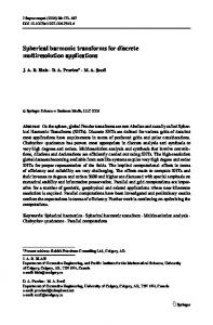
Fig. 1. Results from computation with ∆θ = ½∆λ in REAL*8 Precision on AMD 64 Athlon FX-53 PC. Left:.SHT RMS Values for Synthesis/Analysis [a] and Synthesis [b] of Simulated Series (unit coefficients [RMS1] and 1/degree2 coefficients [RMS2]). Right:.SHT Time Values for Synthesis/Analysis [S/A] and Synthesis [S] of Simulated Series (unit coefficients [TIME1] and 1/degree2 coefficients [TIME2])

9.0E+04

-27.00 8.0E+04 TIME1 [S/A]

-28.00

TIME1 [S] 7.0E+04

TIME2 [S/A]

-29.00

TIME2 [S] 6.0E+04

Time (sec)

Log(RMS)

-30.00 Log(RMS 1a)

-31.00

Log(RMS 1b) Log(RMS 2a)

5.0E+04

4.0E+04

Log(RMS 2b)

-32.00

3.0E+04

-33.00

2.0E+04

-34.00

1.0E+04

0.0E+00

-35.00 0

500

1000

1500

2000

2500

3000

3500

0

4000

500

1000

1500

2000

2500

3000

3500

4000

Degrees and Orders

Degrees and Orders

Fig. 2. Results from computation with ∆θ = ∆λ in REAL*16 Precision on DEC Alpha Computer. Left: SHT RMS Values for Synthesis/Analysis [a] and Synthesis [b] of Simulated Series (unit coefficients [RMS1] and 1/degree2 coefficients [RMS2]). Right: SHT Time Values for Synthesis/Analysis [S/A] and Synthesis [S] of Simulated Series (unit coefficients [TIME1] and 1/degree2 coefficients [TIME2])

anm = 1/(n+1)2,

(14) 2

bnm = 0 for m=0, and 1/(n+1) , otherwise,

(15)

80


for all degrees n and orders m, which simulate a physically realizable situation.Figures 1 show the plots of the RMS values in logarithmic scale and the computation times for double precision computation with grid ∆θ = ½∆λ . The above procedure is repeated for quadruple precision computations and for the grid ∆θ = ∆λ. The results of the RMS values and the computation times are plotted in Figures 2. The analysis and synthesis numerical results in double precision are stable up to approximately degrees and orders 2000, as previously mentioned, and with quadruple precision, the computations are very stable at least up to degree and order 3600. Spectral analysis of the synthesis/analysis results can be done degree by degree to study the characteristics of the estimated spectral harmonic coefficients. The results of the second synthesis also enable a study of the spatial results parallel by parallel, especially for the polar regions. Such investigations are currently underway to better characterize the numerical stability and reliability of the SHT and SHT-1. Ongoing experimentation is attempting to carry out the computations to higher degrees and orders.

6 Concluding Remarks Considerable work has been done on solving the computational complexities, and enhancing the speed of calculation of spherical harmonic transforms. The approach of Driscoll and Healy [5] is exact for exact arithmetic, and with a number of modifications, different implementations have been experimented with, leading to RMS errors of orders 10-16 to 10-12 with unit coefficients of degrees and orders up to 1800. Such RMS errors have been seen to increase to 10-3 with degrees and orders around 2000. With quadruple precision arithmetic, RMS errors are of orders 10-31 to 10-29 with unit coefficients of degrees and orders 3600. Starting with spherical harmonic coefficients corresponding to 1/degree2, the previously mentioned analysis and synthesis results are improved to 10-17-10-16 and 10-35-10-34, respectively. The latter simulations are perhaps more indicative of the expected numerical accuracies in practice. Computations for even higher degrees and orders are under consideration assuming the availability of parallel FFT code in quadruple precision. As enormous quantities of data are involved in the intended gravity field applications, parallel and grid computations are imperative for these applications. Preliminary experimentation with parallel processing in other applications has already been done and spherical harmonic computations appear most appropriate for parallel and grid implement tations.

Acknowledgement The authors would like to acknowledge the sponsorship of the Natural Science and Engineering Research Council in the form of a Research Grant to the first author on Computational Tools for the Geosciences. Special thanks are hereby expressed to Dr. D. Phillips of Information Technologies, University of Calgary, for helping with the optimization of our code for different computer platforms. Comments and suggestions from a colleague, Dr. N. Sneeuw, are also gratefully acknowledged.


81

References 1. Adams, J.C. and P.N. Swarztrauber [1997]: SPHEREPACK 2.0: A Model Development Facility. http://www.scd.ucar.edu/softlib/SPHERE.html 2. Blais, J.A.R. and D.A. Provins [2002]: Spherical Harmonic Analysis and Synthesis for Global Multiresolution Applications. Journal of Geodesy, vol.76, no.1, pp.29-35. 3. Blais, J.A.R. and D.A. Provins [2003]: Optimization of Computations in Global Geopotential Field Applications. Computational Science – ICCS 2003, Part II, edited by P.M.A. Sloot, D. Abramson, A.V. Bogdanov, J.J. Dongarra, A.Y. Zomaya and Y.E. Gorbachev. Lecture Notes in Computer Science, vol.2658, pp.610-618. Springer-Verlag. 4. Colombo, O. [1981]: Numerical Methods for Harmonic Analysis on the Sphere. Report no. 310, Department of Geodetic Science and Surveying, The Ohio State University 5. Driscoll, J.R. and D.M. Healy, Jr. [1994]: Computing Fourier Transforms and Convolutions on the 2-Sphere. Advances in Applied Mathematics, 15, pp. 202-250. 6. Gorski, K.M., E. Hivon and B.D. Wandelt [1998]: Analysis Issues for Large CMB Data Sets. Proceedings of Evolution of Large Scale Structure, Garching, Preprint from http://www.tac.dk/~healpix (August 1998). 7. Górski, K.M., B.D. Wandelt, E. Hivon, F.K. Hansen and A.J. Banday [1999]: The HEALPix Primer, http://arxiv.org/abs/astro-ph/9905275 (May 1999). 8. Healy, D., Jr., D. Rockmore, P. Kostelec and S. Moore [1998]: FFTs for the 2-Sphere Improvements and Variations, To appear in Advances in Applied Mathematics, Preprint from http://www.cs.dartmouth.edu/˜geelong/publications (June 1998). 9. Holmes, S.A. and W.E. Featherstone [2002a]: A unified approach to the Clenshaw summation and the recursive computation of very-high degree and order normalised associated Legendre functions. Journal of Geodesy, 76, 5, pp. 279-299. 10. Holmes, S.A. and W.E. Featherstone [2002b]: SHORT NOTE: Extending simplified highdegree synthesis methods to second latitudinal derivatives of geopotential. Journal of Geodesy, 76, 8, pp. 447-450. 11. Mohlenkamp, M.J. [1997]: A Fast Transform for Spherical Harmonics. PhD thesis, Yale University. 12. Mohlenkamp, M.J. [1999]: A Fast Transform for Spherical Harmonics. The Journal of Fourier Analysis and Applications, 5, 2/3, pp. 159-184, Preprint from http://amath.colorado.edu/faculty/mjm. 13. Mohlenkamp, M.J. [2000]: Fast spherical harmonic analysis: sample code. http://amath.colorado.edu/faculty/mjm. 14. Moore, S., D. Healy, Jr., D. Rockmore and P. Kostelec [1998]: SpharmonKit25: Spherical Harmonic Transform Kit 2.5, http://www.cs.dartmouth.edu/˜geelong/sphere/. 15. Provins, D.A. [2003]: Earth Synthesis: Determining Earth’s Structure from Geopotential Fields, Unpublished PhD thesis, University of Calgary, Calgary. 16. Rapp, R.H. [1982]: A FORTRAN Program for the Computation of Gravimetric Quantities from High Degree Spherical Harmonic Expansions. Report no. 334, Department of Geodetic Science and Surveying, The Ohio State University. 17. Schwarzschild, B. [2003]: WMAP Spacecraft Maps the Entire Cosmic Microwave Sky With Unprecedented Precision. Physics Today, April, pp. 21-24. 18. Sneeuw, N. [1994]: Global Spherical Harmonic Analysis by Least-Squares and Numerical Quadrature Methods in Historical Perspective. Geophys. J. Int. 118, 707-716. 19. Varshalovich, D.A., A.N. Moskalev and V.K. Khersonskij [1988]: Quantum Theory of Angular Momentum. World Scientific Publishing, Singapore. 20. Wenzel, G. [1998]: Ultra High Degree Geopotential Models GPM98A, B and C to Degree 1800. Preprint, Bulletin of International Geoid Service, Milan.