Optimization of the Injection Moulding Process for ... - Sigmasoft

Dr.-Ing. Lothar Kallien. Sigma Engineering GmbH, Aachen. Optimization of the Injection Moulding Process for Thermoplasts With 3D Simulation

Optimization of the Injection Moulding Process for Thermoplasts With 3D Simulation Dr.-Ing. Lothar Kallien Sigma Engineering GmbH, Aachen

Dr.-Ing. Lothar Kallien. Sigma Engineering GmbH, Aachen. Optimization of the Injection Moulding Process for Thermoplasts With 3D Simulation

Optimization of the Injection Moulding Process for Thermoplasts With 3D Simulation

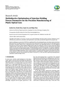
programs always assume parallel laminar flow. Figure 2.1 schematically illustrates zones in a plastic component in which three-dimensional flow effects develop /4/.

1. Introduction The use of innovative CAE technologies has made it possible to drastically reduce the time required for process and product development. A new simulation tool for optimization of thermoset components has recently become available, and can be used for three-dimensional computation of the mould filling, cross-linking and internal stress buildup on a monitor. In contrast to conventional programs, the described program operates with volume elements deriving from the technology of injection moulding of plastics. The frequently three-dimensional geometries of thermoset components are thus depicted in a physically correct sense. The flow algorithm for the filling simulation is based on the Navier-Stokes equations, i.e. kinetic effects such as independent stream formation are predicted. Air inclusions that can result from turbulent mould filling are thus detected at an early stage in mould design and eliminated by optimization. The mould is three-dimensionally networked and the local temperature distribution calculated in the new 3D program. Thus, inhomogeneous temperature zones such as corner effects and their influence on the local cross-linking behavior are taken into account. Multiple cycles can be simulated to determine the temperature distribution in the mould during production startup up to the quasi-stationary state. After stripping, thermally induced internal stresses, particularly as a result of contraction constraints due to metallic inserts, can lead to cracking. The buildup of such internal stress can be calculated and the resultant cracking thus predicted.

Figure 2-1: Zones of three-dimensional melt flow in injection moulding /5/

3. CAD Transference and Cross-Linking in 3D Including Mould and Inserts Presently, volume-oriented CAD data exist for the product to be calculated in most cases. These can be imported into SIGMASOFT® as STL files. All types of FEM volume networks can similarly be transferred to SIGMASOFT®. The geometry of the moulding can be expanded to include the injection points or the mould geometry using an integrated solid modeler. Separation into a three-dimensional volume network is fully automatic. Depending on the complexity of the networking geometry, this operation takes only a few seconds to a maximum of 2 – 3 minutes. In any case, the complete mould including all cooling and heating channels is networked.

4. Simulation of a Thermoset Component A water circulation system produced at LM Plast for a French automobile was simulated in cooperation with the Vyncolit Company. The component is used in PSA-group cars such as the 106, 206 and 306 Peugeot models and the Saxo, Xsara and Berlingo Citroen models (Figure 4-1).

2. 2D and 3D Simulation In developing injection moulded components, simulation programs are used that – based on empirical data and mathematical models - can compute mould filling, the holding and the cooling phase to the point of stripping, and the extent of component deformation /1,2/. Programs used to date for simulation of injection moulding processes rely on geometric information that approximately describes the upper, lower and middle planes of the actual geometry. This method of calculation is generally referred to as a 2?-dimensional shell model. The only approximate description of the component geometry by a middle plane can have a negative effect on the quality of the result. This particularly applies to calculation of components with irregular wall thickness /3,4,5,6/. Furthermore, threedimensional flow effects cannot be resolved, since these

Figure 4-1: Citroen Berlingo

1

Dr.-Ing. Lothar Kallien. Sigma Engineering GmbH, Aachen. Optimization of the Injection Moulding Process for Thermoplasts With 3D Simulation

This involved replacement of a die-cast aluminum component by a thermoset part. One of the reasons for this substitution was the major weight advantage: the aluminum component weighs 614 g, and the plastic part only 344 g. Figure 4-2 shows a direct comparison of the aluminum component (left) and the new thermoset part (right).

Figure 4-4: SIGMASOFT® volume model

Figure 4-2: Comparison of an aluminum (left) and thermoset (right) component

The design geometry was retained essentially unchanged in this simulation. The component is fabricated in a single-cavity mould. The data were adopted from a CAD System, and simply imported into the preprocessor (Figure 4-3).

After the geometry has been entered, the process and material data must be added. These include the filling time, the volume flow or filling pressure at the gate, the temperature of the thermoset material when injected, the preliminary crosslinking density, the mould temperature and information on the thermal conductivity coefficients of the involved groups of materials. The density, thermal conductivity, heat capacity as a function of the temperature and the cross-linking enthalpy of the thermoset must be known. In order to calculate cross-linking as a function of the time, cross-linking curves at a minimum of three different temperatures must be entered into the program. Figure 4-5 illustrates a cross-linking curve for a temperature of 160°C. SIGMASOFT® approximates this process fully automatically using the Deng-Isayev model. The actual results and the approximated cross-linking curve are directly compared in the figure.

Figure 4-3: Transfer of geometry to the simulation

Networking in three-dimensional volume elements is fully automatic. Figure 4-4 shows the networking geometry including the sprue.

Figure 4-5: Cross-linking curve at a temperature of 160°C

The cross-linking reaction during mould filling is also calculated in SIGMASOFT®. This is accomplished using a CrossArrhenius formula that describes the viscosity as a function of the shear rate, the temperature and the local cross-linking den2

Dr.-Ing. Lothar Kallien. Sigma Engineering GmbH, Aachen. Optimization of the Injection Moulding Process for Thermoplasts With 3D Simulation

sity. If the cross-linking density exceeds a critical value in specific zones, the viscosity rises sharply and flow is no longer possible. The following formulas describe this relationship.

Alpha gel is the cross-linking density at which flow is no longer possible. For α ≤ α gel the following term

describes the viscosity as a function of the cross-linking density, the temperature and the shear rate. In this case

and Figure 4-6: Temperature distribution at 85 % mould fill

If α ≤ α gel then

Tb:

Reference temperature

[K]

B:

Arrhenius constant

[Pas]

τ*:

Material constant

[Pa]

n:

Cross exponent

α gel:

Cross-linking density

C1, C2: Constants The process parameters for the component were as follows: • Filling time: 5s • Bulk temperature: 110 °C • Preliminary cross-linking density of the compound during filling: 5 % • Mould temperature: 170 °C

Mould filling, the cross-linking reaction, cooling to ambient temperature and the resultant internal stresses were calculated. Figure 4-6 shows the temperature distribution at 85 % mould fill. The compound enters the heated mould at 110 °C, and the temperature rises further. The local shear rate is highest at the gate (Figure 4-7).

Figure 4-7: Local shear rate distribution in the gate

The flow phenomena can also be visualized using tracer particles. The colors of these weightless particles in Figure 4-8 show the ingress age of the particles, whereas the vectors describe the directions and velocities of the particles. Figure 4-9 shows the temperature distribution at the conclusion of mould filling. The coldest melt is located at the gate.

3

Dr.-Ing. Lothar Kallien. Sigma Engineering GmbH, Aachen. Optimization of the Injection Moulding Process for Thermoplasts With 3D Simulation

Figure 4-8: Tracer particles visualize the flows

Figure 4-10: Local filling times in seconds

Figure 4-9: Temperature distribution at 100% mould fill

Figure 4-11: Pressure distribution at conclusion of filling. The arrow shows the position of the internal pressure sensor in the mould.

The mould filling process can also be described by the local filling time (Figure 4-10). The pressure required for filling is illustrated in Figure 4-11. The value at the front flange (arrow) could be verified by an internal pressure sensor in the mould. A pressure of 230 bars was determined at this point.

Since the compound is injected into the cavity at a preliminary cross-linking density of 5 %, the local cross-linking density has risen to 11 % at the end of the filling operation (Figure 4-12). Particularly in the vicinity of ribs, where the melt can no longer flow, the compound rapidly heats up and begins to cross-link (arrow). The local cross-linking density has increased to 55 % after 16 seconds (Figure 4-13). The effect of mould filling is clearly apparent, since the zones that are farther away from the gate are more highly cross-linked by the elevated temperature.

4

Dr.-Ing. Lothar Kallien. Sigma Engineering GmbH, Aachen. Optimization of the Injection Moulding Process for Thermoplasts With 3D Simulation

Figure 4-12: Local cross-linking density at conclusion of mould filling. Zones such as ribs, which are not exposed to a continuous flow, heat up and cross-link more rapidly.

Figure 4-14: Local cross-linking density after 40 seconds

Figure 4-13: Local cross-linking density after 16 seconds

Figure 4-15: “X-ray” view of zones with less than 70 % cross-linking density

After 40 seconds, 7 % of the total compound is cross-linked (Figure 4-14). Zones with less than 70 % cross-linking can be visualized in an “X-ray” view (Figure 4-15).

Following cross-linking in the mould, cooling in air to ambient temperature is calculated. The thermally induced internal stresses outside the mould can be calculated on the basis of a plastic-elastic material model in order to obtain data on deformation. The stress calculation can be carried out for both isotropic materials and anisotropic, fiber-reinforced thermosets. The stress calculation assumes that the material is completely cross-linked when the mould is opened. The calculation is based on the following temperature-dependent, thermomechanical parameters:

5

Dr.-Ing. Lothar Kallien. Sigma Engineering GmbH, Aachen. Optimization of the Injection Moulding Process for Thermoplasts With 3D Simulation

• The isotropic elastic modulus or the elastic modulus lengthwise and transverse to the fiber direction • The isotropic coefficient of thermal expansion, or the parameter lengthwise and transverse to the fiber direction • The transverse contraction number In this case, the plastic is a short glass fiber-reinforced material. The elastic modulus in such a case depends very greatly on the fiber orientation. The fiber orientation can be three-dimensionally calculated using SIGMASOF®. Figure 4.16 shows the fiber orientation in a rib foot. Figure 4-17 shows the local distribution of the von-Mises internal stresses at ambient temperature. Because of the previously mentioned limitation, the results should be considered qualitative. Figure 4-18 shows the main stresses along the y-axis. The local shifts can be calculated on the basis of these values.

Figure 4-18: Thermally induced main stresses along the y-axis

Figure 4-19 shows the shifts along the y-axis. The depicted degree of deformation is exaggerated by a factor of 50.

Figure 4-16: Three-dimensionally calculated fiber orientation in a rib transition area. The vectors indicate the direction of the fibers, and the colors show the degree of orientation in the pertinent element.

Figure 4-19: Shifts along the y-axis

Figures 4.2x show a direct comparison of filling simulations.

4 Export of Results to FE Networks

Figure 4-17: Thermally induced internal (von-Mises) stresses

Using a new interface, both the cross-linking reaction and fiber orientation results can also be exported to finite element networks. Figure 4.20 shows the three-dimensionally calculated fiber orientation along the xaxis for a test component. This result can now be exported to a wide variety of finite element networks. Figure 4.21 shows the fiber orientation after being exported to a finite element network for further processing in ABAQUS.

6

Dr.-Ing. Lothar Kallien. Sigma Engineering GmbH, Aachen. Optimization of the Injection Moulding Process for Thermoplasts With 3D Simulation

Figure 4-20: 3D-fiber orientation in SIGMASOFT®

Figure 4-22: Direct comparison of the simulation and the result of an experimental filling test shows very good agreement even in details (arrow).

Figure 4-21: 3D-fiber orientation in a finite element network for further processing in ABAQUS

Figure 4.22 shows a direct comparison of the filling simulation with actual filling studies that were later performed. The simulation in the top picture offers an excellent view of the connecting seam in the component.

5. Thermoset Components With Inserts The stress calculations are of particular interest when inserts are to be embedded. Holec Holland NV in Hengelo manufactures thermoset components for high-tension engineering that are exposed to as much as 24 kV in later use. Metallic inserts are embedded in the thermoset of these components. The different coefficients of thermal expansion of the thermoset and the metal can lead to stress cracking that affects the operation of the component. At Holec, the SIGMASOFT® simulation program is used to predict filling, cross-linking and stress buildup during cooling. An optimized design for the component and the mould can thus be developed prior to actual component and mould construction. Figure 5-1 shows the thermoset component, and Figure 5-2 the insert. Figure 5-3 shows the temperature distribution at the conclusion of mould filling. The effect of mould filling on the temperature distribution is also apparent in this component.

7

Dr.-Ing. Lothar Kallien. Sigma Engineering GmbH, Aachen. Optimization of the Injection Moulding Process for Thermoplasts With 3D Simulation

6. Summary Mould filling, cross-linking, cooling and internal stress buildup during fabrication of thermoset components by casting or injection moulding can be three-dimensionally calculated using the new simulation tool. This permits optimization of the component design and mould prior to production. SIGMASOFT® operates on the basis of three-dimensional volume elements. The advantages of this new 3D simulation method using volumetric elements for simulation of thermoset components may be summarized as follows: • Model preparation costs are eliminated since CAD data can be utilized and automatically networked.

Figure 5-1: High-tension component from Holec

• Flow phenomena such as backwater areas in thick-walled zones of mouldings or at points with different wall thickness are described in physically exact terms. • Kinetic effects such as independent stream formation may be predicted. • Calculation of the cross-linking reaction takes account of the reaction enthalpy. • Local cross-linking has an effect on mould filling. • It is possible to take account of the back-pressure of air in the mould. • The fiber orientation can be calculated in three dimensions, and used for stress analysis. • The thermally induced buildup of internal stress during cooling can be calculated. • Thermal effects on the flow and cross-linking processes are accounted for by the three-dimensionally coupled calculation of the moulding, inserts and mould.

Figure 5-2: Metal insert

• The consideration of heating systems is three-dimensional; the local effect on the mould wall temperature is calculated. • The cycle time can be predicted.

References 1. H. Bogensberger, Kunststoffe 85, 44 ff (1995). 2. P.F. Filz, Kunststoffe 88, 954 ff (1998). 3. B. Ohlsson, First International Thermoset Symposium in Iserlohn, Märkische Fachhochschule Iserlohn 4. P. Thienel, International Mould Construction Symposium 1999, Dr. Reinhold Hagen Stiftung, Bonn 5. W. Michaeli, H. Findeisen, and T. Gossel, Kunststoffe 87, 462 ff (1997). 6. O. Altmann and H.J. Wirth, Kunststoffe 87, 1670 ff (1997). Figure 5-3: The temperature distribution at the conclusion of mould filling shows the effect of this operation

7. A.J. van der Lelij, Kunststoffe 87, 51 ff (1997).

8