Jul 31, 2006 - Optimization of the robustness of multimodal networks. Toshihiro Tanizawa,1 Gerald Paul,2 Shlomo Havlin,2,3 and H. Eugene Stanley2.
PHYSICAL REVIEW E 74, 016125 共2006兲
Optimization of the robustness of multimodal networks 1
Toshihiro Tanizawa,1 Gerald Paul,2 Shlomo Havlin,2,3 and H. Eugene Stanley2
Kochi National College of Technology, Monobe-Otsu 200-1, Nankoku, Kochi 783-8508, Japan Center for Polymer Studies and Department of Physics, Boston University, Boston, Massachusetts 02215, USA 3 Minerva Center and Department of Physics, Bar-Ilan University, 52900 Ramat-Gan, Israel 共Received 15 November 2005; published 31 July 2006兲
2
We investigate the robustness against both random and targeted node removal of networks in which P共k兲, the m −共i−1兲 a ␦共k − ki兲 with ki ⬀ b−共i−1兲 and distribution of nodes with degree k, is a multimodal distribution, P共k兲 ⬀ 兺i=1 Dirac’s delta function ␦共x兲. We refer to this type of network as a scale-free multimodal network. For m = 2, the network is a bimodal network; in the limit m approaches infinity, the network models a scale-free network. We calculate and optimize the robustness for given values of the number of modes m, the total number of nodes N, and the average degree 具k典, using analytical formulas for the random and targeted node removal thresholds for network collapse. We find, when N � 1, that 共i兲 the robustness against random and targeted node removal for this multimodal network is controlled by a single combination of variables, N1/共m−1兲, 共ii兲 the robustness of the multimodal network against targeted node removal decreases rapidly when the number of modes becomes larger than a critical value that is of the order of ln N, and 共iii兲 the values of exponent opt that characterizes the scale-free degree distribution of the multimodal network that maximize the robustness against both random and targeted node removal fall between 2.5 and 3. DOI: 10.1103/PhysRevE.74.016125
PACS number共s兲: 89.75.Hc, 02.50.Cw, 64.60.Ak, 89.20.Hh
I. INTRODUCTION
Many real world networks have been found to be scalefree networks, for which P共k兲, the distribution of nodes of degree k, have the form P共k兲 ⬃ k− 关1–11兴. Degree distribution is only one characteristic of networks; in real networks such features as clustering and degree-degree correlations play an important role. Here we consider random graphs with a particular degree distribution and our results apply to such networks. One of the properties of scale-free networks is their robustness against random failure of nodes. At the same time, however, the scale-free network is easy to collapse when a small number of highly connected nodes 共“hubs”兲 are selectively removed. Formally, we define the thresholds, f r and f t, as the fraction of nodes necessary to be removed in order to destroy the giant component of a given network by random and targeted node removal, respectively 关12–17兴. Then f r ⬇ 1 and f t � 1 for scale-free networks 关14–22兴. We define the optimal degree distribution for robustness against both random and targeted node removal as the degree distribution that maximizes the sum of the two critical fractions 共thresholds兲, which is denoted by f T ⬅ f r + f t, for given values of the parameters that specify the network under consideration 关20,23兴. Since f r and f t are bounded by 关0 , 1兴, f T is bounded by 关0 , 2兴. In previous work, the authors determined that the network that is maximally robust against both random and targeted node removal 关20,21兴 is a network characterized by the bimodal degree distribution
冦
k = k1 ⱕ 具k典,
r1 = 1 − r2
冉 冊 2
A P共k兲 = r2 ⬅ 具k典N 0
3/4
where 1539-3755/2006/74共1兲/016125共8兲
k = k2 = 冑具k典N, otherwise,
冣
共1兲
A⬅
再
2具k典2共具k典 − 1兲2 2具k典 − 1
冎
1/3
共2兲
with the average degree 具k典 共see also Ref. 关22兴兲. For this optimal bimodal network, f r ⬇ 1 and f t ⬇ 1 − 1 / 共具k典 − 1兲 with each of these thresholds approaching its theoretical maximum asymptotically as N → ⬁. This bimodal network can be considered to be a network that appears to be consistent with a power-law degree distribution, P共k兲 ⬀ k−, with =−
5 ln r2 + 1 → = 2.5. ln k2 N→⬁ 2
共3兲
Considering that the scale-free network does not have the robustness against targeted removal of nodes that the bimodal network does have, while both of them are equally robust against random removal of nodes, we study how the robustness against targeted node removal is lost as the number of degrees contained in the degree distribution increases. An important question is whether the robustness against targeted node removal is lost gradually or abruptly as we increase the number of degrees contained in the degree distribution. Motivated by this consideration, we investigate the robustness of the networks with a degree distribution specified by m
m
i=1
i=1
P共k兲 = 兺 ri␦共k − ki兲 = 兺 r1a−共i−1兲␦共k − ki兲
共4兲
with ki = k1b−共i−1兲, where ␦共x兲 is Dirac’s delta function. A specific realization of graphs subject to this degree distribution is generated by the classical algorithm in the so-called configuration model 关11–13兴. We refer to this type of network as a scale-free multimodal network. This degree distribution is characterized by three parameters: a that controls the fraction
016125-1
©2006 The American Physical Society
PHYSICAL REVIEW E 74, 016125 共2006兲
TANIZAWA et al.
of nodes having different degrees and is larger than 1, b that controls the values of the degrees and takes a value in the range between 0 and 1, and k1 that is the smallest possible degree. The normalization constant r1 is the fraction of nodes that has the smallest possible degree, k1. The network consists of nodes with m distinct degrees, and we refer to m as the number of “modes.” By varying m, we are able to study the robustness of power-law networks from the bimodal network 共m = 2兲 to the scale-free network 共m → ⬁ 兲 in a unified way. By changing two parameters, a and b, we can determine the values for the optimal network that maximizes the sum of two thresholds, f r and f t, against random and targeted node removal. All calculations for optimization are performed for given values of the total number of nodes N, and for a fixed average degree 具k典. This paper is organized as follows. In Sec. II, we mathematically define the scale-free multimodal network model. In Secs. III and IV, we derive the analytical expressions for the critical removal fractions 共thresholds兲, f r and f t, necessary to destroy the giant component of the multimodal network by random and targeted node removal. In Sec. V, we identify the controlling combination of parameters, N1/共m−1兲. In Sec. VI, we calculate the optimal values of parameters that maximize the sum of the thresholds, f r + f t, and determine the corresponding optimal values of the exponent in the scalefree multimodal degree distribution. In particular, we focus on the behavior of the robustness against targeted node removal as the number of modes m increases in the optimization. Section VII summarizes our results. II. MODEL
The multimodal network of m modes is defined by the degree distribution m
P共k兲 = 兺 ri␦共k − ki兲,
共5兲
i=i
where ␦共x兲 is Dirac’s delta function and ri ⬅ r1a−共i−1兲
共a ⬎ 1; i = 1,2, . . . ,m兲
k i ⬅ k 1b
共0 ⬍ b ⬍ 1; i = 1,2, . . . ,m兲
共7兲
links. The parameter a is a real number larger than 1, and the parameter b is a real number between zero and one. Hence r1 ⬎ r2 ⬎ ¯ ⬎ rm and k1 ⬍ k2 ⬍ ¯ ⬍ km. The degree distribution of the multimodal network obeys a power law P共ki兲 = ri ⬀ k− i ,
共8兲
m
ri = r1 兺 a−共i−1兲 = 1, 兺 i=1 i=1
共10兲
1 − a−1 , 1 − a−m
共11兲
we have r1 =
From the normalization condition
rm =
a−1 , am − 1
a−1 q = . m a −1 N
共12兲
The average degree 具k典 is calculated by m
m
i=1
i=1
具k典 = 兺 kiri = k1r1 兺 共ab兲−共i−1兲 .
共13兲
By fixing the values of 具k典 and k1, this equation determines a relation between a and b. Since the value of a is determined by Eq. 共12兲, we have two free parameters, q and k1, for the optimization of the scale-free multimodal network for given values of m, N, and 具k典. Notice that Eqs. 共12兲 and 共13兲 are both mth order algebraic equations, which we can solve only numerically for m ⱖ 5. III. THRESHOLD fr AGAINST RANDOM FAILURES OF NODES
We consider networks that are simple, i.e., the probability of two edges linking the same pairs of nodes in constructing a network satisfying a given degree distribution is negligible. There is no loss of generality in restricting the networks we consider to be simple because multiple edges linking the same pairs of nodes add nothing to robustness against node removal. The requirement that the network be simple is reflected in the constraint that the largest degree with nonzero probability km must obey kmax ⬅ 冑具k典N.
共14兲
This constraint is valid asymptotically for graphs with a specified degree distribution created randomly using the configuration model 关24–27兴. The threshold against random failures is calculated from the formula suitable for simple graphs 关16,28兴, fr = 1 −
1 , −1
共15兲
where = 具k2典 / 具k典, which can be calculated exactly in our model as
where, as shown in Appendix A, ln a + 1. =− ln b
or
since a ⫽ 1. When the total number of nodes is N and the number of the nodes that have the highest degree km is q, the value of a is determined by the equation
共6兲
is the fraction of nodes that have −共i−1兲
m
= r1
共9兲
k21 1 − 共ab2兲−m . 具k典 1 − 共ab2兲−1
共16兲
The averages are taken over the degree distribution before node removal. The optimal configuration for random 016125-2
PHYSICAL REVIEW E 74, 016125 共2006兲
OPTIMIZATION OF THE ROBUSTNESS OF¼
␣l ⬅ 1 − r1Al + bl−1r1Bl .
共19兲
l Similarly, by defining Cl ⬅ 兺i=1 共ab2兲−共i−1兲, we have
⬘ ⬅
␥l − f lt 具k2典⬘ = kl 具k典⬘ l − f lt
共20兲
with
l ⬅ 1 − r1Al−1 + bl−1r1Bl−1
共21兲
␥l = 1 − r1Al−1 + b2共l−1兲r1Cl−1 .
共22兲
and FIG. 1. Schematic representation of the degree distribution for the scale-free multimodal network and the part of the degree distribution removed by a targeted attack on the higher degree modes between kl and km.
removal only is obtained with a bimodal distribution in which the highest degree nodes have degree kmax 关29兴.
Substituting Eqs. 共18兲 and 共20兲 into Eq. 共17兲, we find that Eq. 共17兲 is just a quadratic equation in terms of f lt: ul共f lt兲2 − vl f lt + wl = 0
ul ⬅ kl − 1,
Here we calculate the threshold f t, that is the fraction of highest degree nodes which must be removed before the network loses its global connectivity. We employ the approach of Refs. 关18,19兴 as follows: In addition to changing the maximum degree of the distribution, the removal of high degree nodes causes another effect—since the links that lead to removed nodes are eliminated, the degree distribution also changes. This effect is equivalent to the random removal of a fraction ˜p of nodes, where ˜p is the ratio of the number of links removed divided by the total number of links before the removal. Since the effect is equivalent to a random removal of nodes, Eq. 共15兲 with f r replaced by ˜p and with calculated after the removal of nodes can then be used to calculate the effect of the link removal. That is, we calculate the threshold against targeted node removal by solving the equation 1 , ⬘ − 1
1 − ˜pl =
with
wl ⬅ ␣l共kl␥l − l兲 −
具k典 , kl
具k典 l . kl
共25兲
共26兲
The threshold f 1t can be easily calculated as f 1t = 1 −
具k典 k1共k1 − 1兲
共27兲
but the calculation of the threshold f lt for 2 ⱕ l ⱕ m is performed numerically because of the complexity of the coefficients 共24兲–共26兲. The threshold against targeted node removal f t is the only solution of Eq. 共23兲 for all l共=1 , 2 , . . . , m兲 that satisfies the inequality
再
共l = 1兲,
1 − r1 ⱕ f lt ⱕ 1 1 − 兺 i=1 ri ⱕ f ⱕ 1 − 兺 i=1 ri l
l t
l−1
共2 ⱕ l ⱕ m兲. 共28兲
V. SCALING RELATION BETWEEN n AND m
The fraction of the highest degree nodes, rm, is related to the parameter a by Eq. 共11兲, which is restated as −1 −1 −1 am − rm a + rm − 1 = 共a − 1兲共am−1 + am−2 + ¯ + 1 − rm 兲 = 0.
共29兲 The trivial solution, a = 1, is excluded because the parameter a should take a value larger than 1 in our model. If we distribute q highest degree nodes in N total nodes,
kl kl 兵共1 − r1Al + bl−1r1Bl兲 − f lt其 = 共␣l − f lt兲 具k典 具k典
rm = 共18兲
共24兲
vl ⬅ kl␥l − l + ␣l共kl − 1兲 −
共17兲
where the prime in ⬘ represents that the average is taken over the degree distribution after the removal of nodes. In addition, we use l to denote the index of the lowest degree nodes removed as shown in Fig. 1. Thus f lt is the removal fraction of nodes necessary to destroy the giant component of the network under consideration when the lowest degree necessary to be removed is kl. Since the calculation of f lt is straightforward but tedious, we describe the detail in Appendix B and only show the outline in the following. l l a−共i−1兲 and Bl ⬅ 兺i=1 共ab兲−共i−1兲, the left By defining Al ⬅ 兺i=1 hand side of Eq. 共17兲 becomes
共23兲
with
IV. THRESHOLD ft AGAINST TARGETED NODE REMOVAL
1 − ˜pl =
共l = 1,2, . . . ,m兲,
q ⬅ N␣−1 , N
共30兲
where we introduce a new exponent ␣ and put q = N␣. For the bimodal network that is the most robust against both random
016125-3
PHYSICAL REVIEW E 74, 016125 共2006兲
TANIZAWA et al.
and targeted node removal, ␣ ⬇ 0.25 as seen from Eq. 共1兲 that states r2 ⬃ N−3/4. The smallest possible value of ␣ is zero that corresponds to q = 1. Thus we expect that 0 ⬍ ␣ ⱗ 0.25. When N is large, Eqs. 共29兲 and 共30兲 yield the asymptotic relation a ⬃ N共1−␣兲/共m−1兲 ,
m
共32兲
i=1
When ab = 1, Eq. 共32兲 becomes 具k典 = mk1r1. From Eqs. 共11兲 and 共31兲, the fraction of the lowest degree nodes r1 for large N becomes r1 ⬇ 1 − N−共1−␣兲/共m−1兲. Thus we have an asymptotic relation 具k典 = mk1 in this case. Since the lowest degree k1 must satisfy the inequality 1 ⱕ k1 ⬍ 具k典, this asymptotic relation implies the inequality 1 ⬍ m ⱕ 具k典, which is incompatible to our model where we choose both 具k典 and m as free parameters. Thus we exclude the solution ab = 1 in the following. Equation 共32兲 can be written also in the form m
具k典 = kmrm 兺 共ab兲i−1 ,
共33兲
i=1
where rm = N␣−1 as stated previously. For the optimal bimodal network, the highest degree km takes the maximum allowable value for the network to be simple, kmax ⬅ 冑具k典N. We assume that km also takes the values of the order of kmax for the scale-free multimodal network with m ⬎ 2. Thus by setting km = kmax, the product ab is determined using Eq. 共33兲 to be 共ab兲m−1 + 共ab兲m−2 + ¯ + 1 =
具k典 具k典 = 冑 k mr m 具k典N · N␣−1
= 冑具k典N1/2−␣ .
共34兲
Assuming ab � 1, we can solve Eq. 共34兲 by considering only the leading term of the left hand side and find ab ⬃ N共1/2−␣兲/共m−1兲 ,
共35兲
which is consistent with the assumption, ab � 1. Using the asymptotic relation for a, Eq. 共31兲, we find the asymptotic relation for b, b ⬃ N共1/2−␣兲/共m−1兲−共1−␣兲/共m−1兲 ⬃ N−1/2共m−1兲 .
共36兲
or lnNb ⬇ −1 / 关2共m − 1兲兴. It is interesting that the exponent ␣ is not present in the asymptotic relation for b. From the two asymptotic relations 共31兲 and 共36兲, we see that the degree distribution for this multimodal network is controlled by a single combination of the total number of nodes N and the mode number m which is N1/共m−1兲, when N � 1. Since we fix the total number of nodes N and observe how the response of the multimodal network to random and targeted node removal varies with mode number m we introduce the “scaled” mode number,
m−1 , log10N
共37兲
which is the inverse of the logarithm of N1/共m−1兲 for the analysis of the results in the following sections.
共31兲
or lnNa ⬇ 共1 − ␣兲 / 共m − 1兲. The asymptotic form for b is derived as follows. The average degree is calculated by Eq. 共13兲, which is restated as 具k典 = k1r1 兺 共ab兲−共i−1兲 .
m* ⬅
VI. OPTIMIZATION OF ROBUSTNESS A. Optimal configuration and thresholds
As is described in Sec. I, we take the sum of the two thresholds, f T ⬅ f r + f t, as a measure for the robustness against both random and targeted node removal and define the optimal degree distribution for robustness as the degree distribution which maximizes the measure f T for given values of the number of modes m, the total node number N, and the average degree 具k典. We adjust two parameters for the optimization; the one is the number of the highest degree nodes, q ⬅ N␣, for which the exponent ␣ should take the value between 0 and 0.25, and the other is the lowest degree, k1, which should take the value between 1 and 具k典. In Fig. 2 we plot the values of logN aopt and logN bopt that optimize the total threshold versus the mode number m. The plots are consistent with the asymptotic relations, Eqs. 共31兲 and 共36兲, for large values of m and N. We also see that the asymptotic relation for a, Eq. 共31兲, with ␣ = 0, provides the upper bound of logN aopt for all values of m and that the asymptotic relation for b, Eq. 共36兲, provides the lower bound of logN bopt for all values of m. In Fig. 3共a兲, we plot the optimal values of the measure f Topt for network collapse in terms of the bare mode numbers m for 具k典 = 2.8. The data are re-plotted in terms of the scaled mode number, m* ⬅ 共m − 1兲 / log10N in Fig. 3共b兲. The collapse of the data on a single curve confirms the validity of the argument in the previous section that m* is the controlling parameter. The results for other values of 具k典 are similar to this plot. The optimal values of the measure, f Topt, decreases from the maxima at m = 2 for every value of N as the number of modes increases. This is because the robustness against targeted node removal rapidly decreases from the maximum value 1 − 1 / 共具k典 − 1兲 at m = 2 as the number of high degree nodes increases due to the increase in mode number, while the robustness against random failure remains the values approximately equal to 1 under increase in mode number, as we can see in Fig. 4. It should be emphasized that the decrease in the sum of thresholds due to this loss of robustness against targeted node removal takes place at rather small values of m of the order of log10N. We define the critical scaled mode number m*c for a given value of 具k典, as the average of the values of the scaled mode number at which the profiles of the optimal total thresholds change for given values of the total number of nodes N. For example, the critical scaled mode number m*c for 具k典 = 2.8 is approximately 0.7 关see Fig. 3共b兲兴. When the scaled mode number is larger than m*c , the scale-free multimodal network becomes very fragile against targeted attacks and thus behaves essentially like the scale-free network. In the following, we concentrate on the behavior of important quantities
016125-4
PHYSICAL REVIEW E 74, 016125 共2006兲
OPTIMIZATION OF THE ROBUSTNESS OF¼
FIG. 2. 共a兲 The dependence of the values of lnNaopt for the values of a that maximize the total thresholds on the total number of modes m. The thick curve stands for 1 / 共m − 1兲. 共b兲 The dependence of the values of lnNbopt for the values of b that maximize the total thresholds on the total number of modes m. The thick curve stands for −1 / 2共m − 1兲.
for the scaled mode number smaller than the critical value, m*c . In Fig. 5, we plot the behavior of the exponent ␣, which is defined as logN qopt, and the behavior of the highest degree opt , for the optimal configuration for 具k典 = 2.8 with respect to km the scaled mode number m* smaller than the critical value m*c . The values of ␣ smoothly decrease from the values for the optimal bimodal network, which are approximately equal to 0.25, and reach zero, which is the smallest possible value corresponding to q = 1, at m* = m*c . For the values of the highopt est degree for the optimal configuration the relation km
FIG. 3. 共a兲 Optimal values for the sum of the thresholds, f T ⬅ f r + f t, versus mode number for 具k典 = 2.8 for several values of N. 共b兲 The optimal values for the measure, f Topt, for 具k典 = 2.8 are replotted in terms of the scaled mode number m* ⬅ 共m − 1兲 / log10N. The collapse of the data on a single curve is seen. The curve changes its profile at a certain value of m*, which is about 0.7 for 具k典 = 2.8, and the value is denoted by m*c .
⬇ kmax = 冑具k典N always holds. This fact supports the assumption we made for the derivation of the asymptotic relation for b 关see Eq. 共36兲兴. B. Critical mode number
The multimodal network loses robustness against targeted node removal at m*c . We perform the least square fit for the values of m*c and find the fit m*c = 共0.62 ± 0.015兲具k典 − 共1.0 ± 0.038兲
共38兲
as seen in Fig. 6. Therefore in order to make the multimodal network robust against both random failure and targeted node removal for given values of N and 具k典, the number of modes should be kept lower than the critical mode number mc calculated using the formula
FIG. 4. The values for the threshold against random node removal f r and the threshold against targeted node removal f t for the optimal configuration for 具k典 = 2.8 are plotted in terms of the scaled variable m* ⬅ 共m − 1兲 / log10N for 0 ⬍ m* ⬍ m*c ⬇ 0.7.
016125-5
PHYSICAL REVIEW E 74, 016125 共2006兲
TANIZAWA et al.
FIG. 5. The behavior of the exponent ␣, which is defined as lnNqopt, where qopt is the number of the highest degree nodes, and opt the behavior of the highest degree km for the optimal configuration for 具k典 = 2.8 in terms of the scaled mode number m* smaller than the critical value m*c ⬇ 0.7. The values of ␣ smoothly decrease from the values for the optimal bimodal network, which are approximately equal to 0.25, and reach zero, which is the smallest possible value corresponding to q = 1, at m* = m*c . For the values of the highest opt degree for the optimal configuration the relation km ⬇ kmax * * ⬅ 冑具k典N holds for 0 ⬍ m ⬍ mc .
mc = 1 + 共0.62具k典 − 1.0兲log10N derived from Eqs. 共37兲 and 共38兲. If, e.g., we take N = 108 and 具k典 = 2.5, then mc ⬇ 5.
FIG. 7. The exponent in the multimodal degree distribution for the optimal configuration opt for the scale-free multimodal degree distribution, versus the scaled variable m* ⬅ 共m − 1兲 / log10N of Eq. 共37兲. Note that, as argued in Sec. VI C, the values of opt reside mainly in the interval between 2.5 and 3.
asymptotic relations for a and b, Eqs. 共31兲 and 共36兲, holds. Since Eq. 共31兲 gives the upper bound for a and Eq. 共36兲 gives the lower bound for b, the 共asymptotic兲 upper bound for opt, which is denoted by ¯opt, is calculated as ¯opt = 1 − 1/共m − 1兲 = 3. − 1/2共m − 1兲
C. Optimal values of the exponent in the degree distribution
The exponent in the multimodal degree distribution for the optimal configuration opt, is calculated by opt = 1 −
ln a . ln b
For the lowest value of m = 2, we have shown in Sec. I that the value is 2.5 关see Eq. 共3兲兴. For large values of N, the
Thus we can conclude that the exponents for the optimal multimodal network take the values within the interval 2.5 and 3. In Fig. 7, we plot the values of opt in terms of the scaled mode number m*. Since for m* ⬎ m*c the scale-free multimodal network effectively loses its discreteness, we only plot the data for m* ⬍ m*c . VII. SUMMARY
FIG. 6. The dependence of the critical values of the scaled mode number m*c on the average degree 具k典. The value of m*c for each 具k典 is the average over all m*c for different values of the total node number N. The critical value m*c is the value of the scaled mode number at which the scale-free multimodal network completely loses its robustness against targeted node removal. The broken line is the fit m*c = 0.62具k典 − 1.0.
In summary, we define and investigate the robustness of scale-free multimodal networks, built as random graphs with a particular degree distribution, against random and targeted node removal and find the optimal configuration for the degree distribution of the scale-free multimodal network for given values of the total number of nodes N and the average degree 具k典 for each value of the mode number m. We find the following: 共i兲 The robustness for a fixed value of the average degree 具k典 depends only on the “scaled” mode number, m* ⬅ 共m − 1兲 / log10N. 共ii兲 The robustness against targeted node removal rapidly decreases as the mode number increases, and effectively becomes zero at a critical value of the scaled mode number, which is m*c = 0.62具k典 − 1.0 for a given value of 具k典. 共iii兲 As the robustness against targeted node removal decreases, the values of the exponent opt that appear in the degree distribution of the scale-free multimodal network varies from 2.5 to 3. Our work should be of value in designing a scale-free multimodal network which is robust to both ran-
016125-6
PHYSICAL REVIEW E 74, 016125 共2006兲
OPTIMIZATION OF THE ROBUSTNESS OF¼
dom and targeted attacks. The network designer must take care not to have the number of different degrees exceed m*c .
APPENDIX B: DETAIL OF THE CALCULATION OF f lt
For the calculation of the ratio of the links removed by the targeted attack ˜pl, we have
ACKNOWLEDGMENTS
We thank ONR for support. One of the authors 共T.T.兲 also thanks the Japan Society for the Promotion of Science for support through a Grant-in-Aid for Scientific Research.
To find a relationship between the multimodal degree distribution and the scale-free degree distribution, we should consider the multimodal P共ki兲 as made up from the corresponding scale-free distribution Psf共k兲 共=Ck−兲 by adding up the number of nodes within a range whose width is ⌬i: P共ki兲 =
冕
Psf共k兲dk = C
冋冉
再
k dk
C 1− k −1 i
再冉 冊 冉 冊 冎 1−
⌬i ki
1−
− 1+
⌬i ki
冊
兺
k ir i
i=l+1 l
冎
l
l
l t
冎
册 共B1兲
.
For the average degree after the removal of nodes, we have
冉
l−1
l−1
具k典⬘ ⬀ 兺 kiri + kl 1 − 兺 ri − f i=1
共A1兲
−
l
m
+
ki kl =1− 1 − 兺 ri + 兺 ri − f k 具k典 i=1 i=1 l
冉兺 l−1
ki−⌬i
ki−⌬i
=
冕
ki+⌬i
1 kl f lt − 1 − 兺 ri 具k典 i=1
1 = kl f lt − 1 + 兺 ri + 具k典 − 兺 kirk 具k典 i=1 i=1
APPENDIX A: RELATION TO THE SCALE-FREE DEGREE DISTRIBUTION
ki+⌬i
再 冋 冉 冊册 l
˜pl =
= kl
i=1
1−
i=1
l−1
ki ri + 1 − 兺 ri − f kl i=1
l t
冊 冊
l t
= kl兵共1 − r1Al−1 + bl−1r1Bl−1兲 − f lt其 = kl共l − f lt兲.
.
共A2兲
共B2兲
Since our values of ki are distributed in k space on an exponential scale, ⌬i has almost the same order of magnitude of ki. In this case 关⌬i = O共ki兲兴,
For the average of squared degree after the removal of nodes, we have
冉 冊 冉 冊 ⌬ 1− ki
1−
⌬ − 1+ ki
l−1
具k 典⬘ ⬀ 兺 2
1−
= O共1兲.
共A3兲
再
+
k2l
i=1
= k2l
Thus ⬘ ⬀ k1− . P共ki兲 ⬀ k− i i
k2i ri
共A4兲
k21
冉
l−1
1 − 兺 ri − f i=1
l t
冊
l−1
2 −共i−1兲 + 1 − Al−1 − f 2 r1 兺 共ab 兲
kl
i=1
l t
冎
= k2l 兵共1 − Al−1 + b2共l−1兲r1Cl−1兲 − f lt其 = k2l 共␥l − f lt兲. 共B3兲
Therefore ⬘ = − 1.
共A5兲
关1兴 A.-L. Barabási and R. Albert, Science 286, 509 共1999兲. 关2兴 M. Faloutsos, P. Faloutsos, and C. Faloutsos, Comput. Commun. Rev. 29, 251 共1999兲. 关3兴 A.-L. Barabási, R. Albert, and H. Jeong, Physica A 281, 69 共2000兲. 关4兴 A. Broder, R. Kumar, F. Maghoul, P. Raghavan, S. Rajogopalan, R. Stata, A. Tomkins, and J. Wiener, Comput. Netw. 33, 309 共2000兲. 关5兴 H. Ebel, L.-I. Mielsch, and S. Bornholdt, Phys. Rev. E 66, 035103共R兲 共2002兲. 关6兴 R. Albert and A.-L. Barabási, Rev. Mod. Phys. 74, 47 共2002兲. 关7兴 M. E. J. Newman, SIAM Rev. 45, 167 共2003兲. 关8兴 H. Jeong, B. Tombor, R. Albert, Z. N. Oltvai, and A.-L. Barabási, Nature 共London兲 407, 651 共2000兲. 关9兴 S. N. Dorogovtsev and J. F. F. Mendes, Evolution of Networks: From Biological Nets to the Internet and the WWW 共Oxford
Equations 共B2兲 and 共B3兲 lead to Eq. 共20兲.
University Press, Oxford, 2003兲. 关10兴 R. Pastor-Satorras and A. Vespignani, Evolution and Structure of the Internet: A Statistical Physics Approach 共Cambridge University Press, Cambridge, England, 2004兲. 关11兴 M. E. J. Newman, in Handbook of Graphs and Networks: From the Genome to the Internet, edited by S. Bornholdt and H. G. Schuster 共Wiley-VCH, Berlin, 2003兲, pp. 35–68. 关12兴 M. Molloy and B. Reed, Random Struct. Algorithms 6, 161 共1995兲. 关13兴 M. Molloy and B. Reed, Combinatorics, Probab. Comput. 7, 295 共1998兲. 关14兴 R. Albert, H. Jeong, and A.-L. Barabási, Nature 共London兲 406, 378 共2000兲. 关15兴 V. Paxon, IEEE/ACM Trans. Netw. 5, 601 共1997兲. 关16兴 R. Cohen, K. Erez, D. ben-Avraham, and S. Havlin, Phys. Rev. Lett. 85, 4626 共2000兲.
016125-7
PHYSICAL REVIEW E 74, 016125 共2006兲
TANIZAWA et al. 关17兴 D. S. Callaway, M. E. J. Newman, S. H. Strogatz, and D. J. Watts, Phys. Rev. Lett. 85, 5468 共2000兲. 关18兴 R. Cohen, K. Erez, D. ben-Avraham, and S. Havlin, Phys. Rev. Lett. 86, 3682 共2001兲. 关19兴 R. Cohen, K. Erez, D. ben-Avraham, and S. Havlin, in Handbook of Graphs and Networks, edited by S. Bornholdt and H. G. Schuster 共Wiley-VCH, New York, 2002兲, Chap. 4. 关20兴 G. Paul, T. Tanizawa, S. Havlin, and H. E. Stanley, Eur. Phys. J. B 38, 187 共2004兲. 关21兴 T. Tanizawa, G. Paul, R. Cohen, S. Havlin, and H. E. Stanley, Phys. Rev. E 71, 047101 共2005兲. 关22兴 A. X. C. N. Valente, A. Sarkar, and H. A. Stone, Phys. Rev. Lett. 92, 118702 共2004兲. 关23兴 As is described in Ref. 关20兴, the general nature of our results hold if we take a linear combination of f r and f t, which is
关24兴 关25兴 关26兴 关27兴 关28兴 关29兴
016125-8
af r + bf t, as a measure, where a and b allow one to specify for a given network the weight to be attached to random and targeted attack respectively. The only modification to our results for these alternative measures, is that the prefactor A, Eq. 共2兲, is multiplied by 共a / b兲1/3. F. Chung and L. Lu, Ann. Comb. 6, 125 共2002兲. Z. Burda and A. Krzywicki, Phys. Rev. E 67, 046118 共2003兲. M. Boguñá, R. Pastor-Satorras, and A. Vespignani, Eur. Phys. J. B 38, 205 共2004兲. M. Catanzaro, M. Boguñá, and R. Pastor-Satorras, Phys. Rev. E 71, 027103 共2005兲. G. Paul, S. Sreenivasan, and H. E. Stanley, Phys. Rev. E 72, 056130 共2005兲. G. Paul, S. Sreenivasan, S. Havlin, and H. E. Stanley, e-print cond-mat/0507249, Physica A 共to be published兲.