Optimization via Simulation of Catchment Basin ...

Simulation

Optimization via Simulation of Catchment Basin Management using Discrete-Event Approach

000(00):1–13 ©The Author(s) 2010 Reprints and permission: sagepub.co.uk/journalsPermissions.nav DOI:doi number http://mms.sagepub.com

J.F. Santucci and L. Capocchi∗ SPE UMR CNRS 6134 Laboratory, University of Corsica, Quartier Grimaldi, 20250, Corte, France

Abstract This paper deals with discrete-event simulation based on optimization of a catchment basin management. The integration of optimization techniques into modeling and simulation relies on the evolution of the studied model using decisions based on previous simulation results. Three different categories of optimization via simulation methods can be found in the literature: rank-and-selection methods, discrete and continuous optimization via simulation methods. In this paper, we explain how an iterative process allows us to integrate continuous optimization via simulation algorithms into a discrete-event simulation in order to optimize the management of a catchment basin. We have performed a comparison between optimization methods belonging to the three categories of optimization via simulation methods when they are applied to the management of a catchment basin. An analysis of the comparison allows us to point out the benefits of discrete-event modeling and simulation coupled with continuous optimization via simulation methods. Keywords optimization methods, discrete-event simulation, discrete-time simulation, simulation software, DEVS, OvS, water management

1. Introduction Modeling and simulation are widely used in research and industry in order to study the behavior of complex systems. These studies include tasks such a: planning, prediction, prevision, computer aided design, etc. When people want to improve the performance of a studied system, the modeling and simulation phases are integrated with an optimization technique. The integration of optimization methodologies into modeling and simulation relies on the evolution of the model using decisions based on previous simulation results by [2, 19, 3]. Usually, the evolution is performed manually by a specialist of the domain. Therefore, it is natural to try to find the set of parameters that optimizes the system performance. This process is called optimization via simulation (OvS). Depending on the format of the parameters (also called decision variables), three main categories of OvS methods may be highlighted: (i) rank-and-selection category (R&S) [26, 25]; (ii) discrete OvS category (DOvS) [33, 45]; (iii) continuous OvS category (COvS) [8, 14, 1].

∗ This

research work was supported by the RESMAR Marittimo European project (http://www.maritimeit-fr.net/). Corresponding author; e-mail: [email protected]

2

Journal name 000(00)

Furthermore, two types of simulation have to be considered: discrete-time (DT) simulation and discrete-event (DE) simulation. Discrete-time simulation leans on the following basic concept: it checks and computes the system states in uniform time increments. The system state variables are computed and updated at regular intervals. Discrete-event simulation leans on the following basic concept: it progresses each time an event occurs. The OvS methods will of course depend on the type of simulation models they have to manage. The two first OvS methods (R&S and DOvS) are linked with DT simulation while the last one COvS is linked with DE simulation. In this paper we are interested in proposing an optimized management of a catchment basin involving dams, power station, pump station, valves, conducts, etc. This management optimization is performed by an automatic integration of optimization techniques into an discrete-event modeling using the DEVS (Discrete Event system Specification) [46] formalism. This paper presents in detail how the behavior of the management of such a complex catchment basin is realized using the DEVS modeling leading to a DE simulation. It describes then how an integration of an COvS optimization technique into the modeling scheme allows to automatically obtain an optimized management of the basin. Three different kinds of optimization methods have been implemented based on the three OvS categories pointed out previously. The R&S method optimization has already been presented in [38] while the DovS optimization method is described in [10, 18, 9]. Both of them are based on a DT simulation approach. In this paper we detailed the optimization of the catchment basin management using a COvS method based on a DE simulation approach. The optimized system has been defined with the DEVS formalism and implemented using DEVSimPy framework [28]. The rest of the paper is as follows. The next section presents in detail the background of this study. The OvS domain is introduced and the main commercial simulation tools including an optimization module are presented. Section 2 also introduced the DEVS formalism and the DEVSimPy framework. In section 3 we detail in the one hand why the DEVS formalism has been chosen and on the other hand why the DEVSimPy modeling and simulation framework has been used in order to implement the DEVS based OvS approach for catchment basin management optimization. Section 4 introduces the case study: the management of a catchment. The problematic associated with the management of catchment basin is clearly stated. Then the DEVS based discrete-event modeling of the case study is detailed and the DEVSimpy implementation introduced. In section 5 we describe how we have realized the optimization of the catchment basin management by developing an COvS approach. The DESVimPy implementation and the results based on the proposed optimization method are presented. Section 6 is dedicated to the analysis and discussion of the proposed approach. We compare the results introduced in section 5 with results obtained when applying R&S and DOvS approaches. Finally, conclusions are given in the last section.

2. Background In this section we introduce the optimization via simulation (OvS) domain. We point out the main categories of methods which can be found under the name of OvS and we introduce a set of existing simulation tools which include an optimization technique. We also introduce the DEVS formalism which has been widely used within modeling and simulation to design, verify, and implement complex reactive systems.

2.1. Optimization via simulation Optimization via simulation is a structured approach to determine optimal settings for input parameters (i.e., the best system design), where optimality is measured by a function of output variables associated to a simulation model [41]. One of the main features of simulation is that one can change the parameters of a simulation model easily and try to observe the system performance under different sets of parameters. Therefore, it is natural to try and find the set of parameters that

Running head right side

3

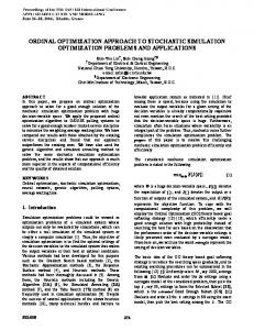
optimizes the system. This set of parameters are determined using an optimization model after evaluating an objective function. Figure 1 depicts the coordination between the optimization model and the simulation model.

Fig. 1. Coordination between the optimization and simulation models.

For a recent comprehensive review of the research and practice of OvS see [20, 21]. Depending on the format of the decision variables vector x, we may divide OvS problems into three categories [24]: •

R&S category: the numerical decision variable set has a small number of potential solutions. Then, we may simulate all solutions and select the best among them. This problem is known as the ranking-and-selection (R&S) problem [40]. R&S procedures evaluate exhaustively all members from a given (fixed and finite) set of alternatives [25].

•

DOvS category: the set of decision variables is discrete and integer ordered. This problem is known as the DOvS problem [43]. A set of algorithms based on the principles of Branch and Bound (BB) [45, 44] approach can be exploited when performing DOvS approach. One of the best known is the dichotomy algorithm. BB algorithms are based on a systematic enumeration of all candidate solutions, where large subsets of fruitless candidates are discarded, by using upper and lower estimated bounds of the quantity being optimized.

•

COvS category: the set of decision variables is a vector of continuous decision variables. This problem is known as the continuous OvS (COvS) problem. In this category the decision variables are continuous and the definition set of these variables is uncountable and infinite. This optimization category has been widely studied and several methods can be pointed out: (i) Stochastic Approximation (SA) [14]; (ii) Metamodel-based optimization algorithm [4]. A set of commercial simulation tools have integrated OvS software modules:

•

Arena simulation [37]: is the most used tool for simulation of discrete-event systems. It is an integrated graphical simulation environment including resources for modeling, design, process visualization, statistical analysis. It integrates the OptQuest [17] for Arena package, which is an optimization tool that is customized for analyzing and optimizing the results of simulation runs, conducted in Arena.

•

Witness [42]: is a process simulation software commonly used for both educational and business purposes, and it is one of the most suitable for simulating plant layouts. The Witness simulation package offers an optimization suite within its experimental framework.

•

Anylogic [7]: is a simulation tool that supports all the most common simulation methodologies: system dynamics, discrete event, and agent based modeling. AnyLogic optimization is built on top of the OptQuest Optimization Engine.

•

Simio [34]: is a powerful discrete-event simulation platform. The modeling aspect are easy to use thanks to a library of intelligent 3D objects. With Simio, complex systems can intuitively be modeled. OptQuest for Simio is available as an add-on to the standard Simio products.

•

AutoMod [32]: is used to create discrete-event simulation models of manufacturing systems, assembly lines, warehouses, distribution centers, airports, and equipment. It is used to: (i) run “what-if” scenarios in a simulation environment to predict results; (ii) analyze and optimize alternate system design concepts based on the AutoStat optimization package. A review of the optimization packages found in commercial simulation software (AutoStat, OptQuest and the Witness

optimizer)reveals that these packages are based on multi-objective optimization routine. AutoStat approaches the multiobjective optimization problem using the classical method in which multiple objectives are aggregated to form a single

4

Journal name 000(00)

objective using a weight-vector. The drawback of this method is that for different decision scenarios, different weightvectors have to be used and the same problem has to be solved repetitively. OptQuest also employed a similar approach. In a same way, Witness optimizer uses Simulated Annealing (SA) and elements of Tabu search are incorporated into the SA process. We can point out that most of the commercial OvS packages implement robust meta-heuristics. For instance, AutoStat uses evolution strategies; OptQuest uses scatter search, Tabu search and artificial neural networks and Witness optimizer uses SA and Tabu search. These meta-heuristics are often robust and perform well on deterministic problems. However they may face problems when random aspects are presents.

2.2. DEVS formalism The DEVS (Discrete Event System Specification) formalism introduced by the Professor Zeigler [46] provides a mean of specifying a mathematical object called a system. Basically, a system has a time base, inputs, states, outputs, and functions for determining next states and outputs given current states and inputs. DEVS provides a formal representation of discreteevent systems capable of mathematical manipulation just as differential equations serve this role. Furthermore, by allowing an explicit separation between the modeling phase and simulation phase, the DEVS formalism is an efficient way to perform simulation of complex systems using a computer. The DEVS formalism procures an Experimental Frame (EF) [29] that specifies conditions under which the system is experimented and observed.

Fig. 2. The DEVS experimental frame.

As illustrated in Fig. 2, an EF has three components: a Generator in charge of generating a set of inputs segments for the system; an Transducer in charge of observing and analyzing the output segments of the system and an Acceptor in charge of selecting the desired data of the system and verifying if the experimental conditions are fulfilled. In the DEVS formalism, in order to model a system, one must specify: (i) basic models from which larger ones are built and (ii) how these models are coupled together in hierarchical order. An atomic model (AM) allows specifying the behavior of a basic element of a given system. Coupling between different atomic models can be defined using a coupled model (CM). An atomic DEVS (AM in Fig. 3) model can be considered as an automaton with a set of states S and transition functions allowing the state change when an event occurs or not.

Fig. 3. The DEVS atomic model.

When no events occur, the state of the atomic model can be changed by an internal transition function called δint . When an external event Xi occurs, the atomic model can intercept it and change its state by applying an external transition

Running head right side

5

function called δext . The life time of a state is determined by a time advance function called ta . Each state change can produce output event Yi via an output function called λ. A coupled model, tells how to couple (connect) several component models together to form a new model. This latter model can itself be employed as a component in a larger coupled model, thus giving rise to hierarchical construction.

Fig. 4. Hierarchical modeling using DEVS coupled models.

Figure 4 depicts an example of the hierarchy between sub-models of a system. The CM0 coupled model represents the system at the highest possible hierarchical level. It has two output ports OUT0 and OUT1, one input port IN and it contains two atomic models AM0 and AM1 but also one coupled model CM1. The two atomic models AM0 and AM1 are coupled with an input external coupling relation with CM0 and with an internal coupling relation with CM1. The output external coupling relation occurs between the two output ports of CM1 and the two output ports OUT0 and OUT1. A simulator is associated with the DEVS formalism in order to exercise instructions of atomic model to actually generate its behavior. The architecture of a DEVS simulation system is derived from the abstract simulator concepts [46] associated with the hierarchical and modular DEVS formalism. One of the advantages of the DEVS formalism is that the simulator is generated automatically from the model. There are many tools which provide a user interface dedicated to help the user to define DEVS models and to perform simulations. A non exhaustive list can be done: PowerDEVS [5], DEVSim++ [27], DEVSJAVA [39], VLE [36], DEVSimPy [28], CD++Builder [6], ATOM3 [12], MS4Me [11], etc. Special attention will be given to DEVSimPy (stand for DEVS simulator in Python language) which is a collaborative modeling and simulation (M&S) software. It is used in order to model and simulate complex systems based on the DEVS formalism with the Python programming language. In particular, DEVSimPy [28] is an open source project with the aim of providing a GUI for the modeling and simulation of PyDEVS models. PyDEVS is an Application Programming Interface (API) allowing the implementation of the DEVS formalism in Python language. Python is known as an interpreted, very high-level, object-oriented programming language widely used to quickly implement algorithms without focusing on the code debugging [35]. The basic idea behind DEVSimPy is to wrap the PyDEVS API with a GUI allowing significant simplification of handling PyDEVS models (like the coupling between models or their storage). With DEVSimPy, DEVS models can be stored in dynamic libraries in order to be reused and shared. A DEVSimPy model can be stored locally in the hard disk or in cloud through the web in the form of a compressed file including the behavior and the graphical view of the model separately. The behavior of the model can be extended using specific plug-ins embedded in the DEVSimPy compressed file. This functionality is powerful since it makes it possible to implement new algorithms above the DEVS code of models in order to extend their handling in DEVSimPy (exploit behavioral attributes, overriding of DEVS methods, ...). A plug-in can also be global in order to manage several models through an generic interface embedded in DEVSimPy. In this case, the general plug-in can be enabled/disabled for a family of selected models. An interesting global plug-in called Blink has been implemented to facilitate the debugging in DEVSimPy. This plug-in is based on the step by step of the simulation and blink the models to indicate their activity with a color code corresponding to the nature of the DEVS transition function (internal, external, time advance, output).

6

Journal name 000(00)

Fig. 5. The DEVSimPy general interface.

Figure 5 gives an example of the window interface. You may notice that the window is split into two parts: (i) the left part (circle 1 in Fig. 5) allows the user to visualize the classes of models which can be instantiated using a drag-and-drop; (ii) the right part (circle 2 in Fig. 5) which is dedicated to the design of coupled models (also called diagrams in the following) with a simple drag-and-drop of classes belonging to the left part of the window. The created coupled model can be saved under a specific format allowing it to be easily reused and shared.

3. OvS in discrete-event simulation context In this sub-section we address OvS in discrete-event simulation context by expliciting why the DEVS formalism has been chosen and why the DEVSimPy tool has been used instead of a commercial tool.

Why DEVS formalism for OvS approach? A set of different formalisms can be used when modeling complex systems. We can mention: DAE, Bond Graph, Forrester System Dynamics, Petri Nets, Finite State Automata, DEVS, State Charts, Queueing networks, etc. The choice of appropriate formalisms depends on criteria such as the application domain, the background of the modeler, the goals, and the available computational resources, etc. [13]. The DEVS formalism has been chosen in the framework of this optimization work for at least two reasons: (1) due to the discrete-event based specification given by hydrologic experts of the CAW agency, the choice of a discrete-event formalism is obvious even though a traditional approach would have been based on a discretetime formalism. (2) it has been highlighted in [13] that it is possible to map all formalisms, and in particular continuous ones, onto DEVS. The DEVS formalism framework of modeling and simulation proposed by the professor Zeigler in [46] offers concepts that are important for the integration of optimization methods in a discrete-event simulation tool: (i) there is an explicit separation between the model and the context under which it is experimented with; (ii) there is a separation between the simulator and the simulation model. This DEVS formalism framework is therefore a good basis for the detailed formalization of the structural relationships between simulation and optimization techniques.

Why DEVSimPy tool as OvS framework? Among the set of DEVS formalism software environments (sub-section 2.2), some of them integrate optimization via simulation methods. We can highlight the following work: •

Simulation Based Parameter and Structure Optimization of Discrete Event Systems presented in [22]: this work provides optimization through automatic reconfiguration of both the model structure and model parameters; the associated

Running head right side

•

7

optimization method uses an evolutionary algorithm integrated through a combination of DEVS formalism and system entity structure/model base framework. The multi-objective evolutionary optimization (SIMEON) framework [23]: the integration of simulation and optimization techniques is performed using the concept of experimental frame [29] formalized with three components which govern the experimentation on a model: the generator, the transducer and the acceptor. SIMEON integrates Genetic algorithm optimization and plans to extend the optimization techniques with different evolutionary based algorithms. The integration is essentially based on the definition of a controller atomic model which controls the whole simulation process. Obviously, this controller model depends on the studied application.

•

A Devs-Based Optimization via Simulation [29]: this work proposes a DEVS-based framework for simulation optimization and provides a proof-of-concept employing DEVSJAVA with an application of Link-11 gateway.

The previous work points out how DEVS environments are able to integrate optimization techniques. These three kinds of frameworks allow to perform optimization via simulation using the DEVS formalism: the two first one integrate global optimization methods based on evolutionist algorithms while the third one proposes an integration based on Experimental Frame and a dynamic variable structure validated on a real case study. We chose to provide a discrete-event OvS approach using the DEVSimPy tool for solving the problem of catchment basin management optimization. We have already pointed out the interest in choosing the DEVS formalism and we have decided to use the DEVSimPy environment in order to integrate a COvS method for the following reasons: (i) the simulation model had already been realized using the DEVSimPy framework - the basic model which is used as a basis for optimization has been realized using the DEVSimPy environment in collaboration with the hydrologic experts of the CAW agency - ; (ii) the discrete-event simulation based on the python language as in DEVSimPy allows to take into account with continuous inputs which are required when dealing with catchment basin management ; (iii) DEVSimPy is supported by the team of the SPE UMR CNRS 6134 laboratory.

4. Case study: Catchment basin management 4.1. Problematic Water is the vital resource to support life on the Corsica Island (island of the Mediterranean area). Unfortunately, it is not evenly distributed over the Island by season or location. Some parts of the island are prone to drought making water a scarce and precious commodity, while in other parts of the island it appears in raging torrents causing floods and loss of life and property. The Corsican Water Agency (CWA) is a governmental institution in charge of distribution and quality of water resources and water bodies, including manmade water infrastructures. CWA manages a complex network of dams, storages and pipelines to provide an adequate supply of water to its customers. Furthermore, in addition to water supply the benefits of this management include also hydropower production. The difficulty when managing a water network [30, 31, 15] involving dams, power stations, pump stations, pipelines, valves is to ensure the water distribution to consumers while the production of electricity using power stations is the highest possible and the use of pump stations is as low as possible. It is the case actually in the south-east of Corsica Island where a water network involves two interconnected dams (Ospedale and Figari), a power station (upstream to the Ospedale dam), a pump station (used in order to send the water taken from Figari dam to the consumers) and a set of valves allowing to send the water from the Ospedale dam to the Figari dam or the consumers (Fig. 1). We have to point out that the south-east region of Corsica has the following features: (i) a lot of rainfall in winter while a drought period in summer ; (ii) the consumer population is multiplied by 10 in summer season (due to tourism) compared to the winter season. Because of this dichotomy between summer and winter, two different behaviors for the management of the network have been defined by the CWA experts:

8

Journal name 000(00)

•

the winter behavior: since the rainfalls are heavy and the population is low, only the Ospedale dam is used fulfill the water supply for the consumers (since the use of the Figari dam requires electricity consumption due to the pump station associated with the dam) and the power station is able to produce electricity when the Ospedale dam is quite

•

full (since the water used by the power station is lost for water supply). the summer behavior: The power station is no more used; the Ospedale dam is first used to fulfill the consumer water supply; when it is quite empty the pump station is then used in order to send water taken from the Figari dam to the consumer.

The hydrology experts belonging to the CWA have defined a management strategy based on the definition of two dates (let us call them d1 and d2) allowing to perform the winter behavior from date d2 to date d1 and then switch to the summer behavior from d1 to d2. However the difficulty for the expert is to find the best dates (d1 and d2) as well as the best amount of turbine water allowing to respect the following three constraints: (i)to respond to the water demand of the consumer all along the year ; (ii) to use as much as possible the power station associated with the Ospedale dam ; (iii) to use as less as possible the pump station associated with the Figari dam. In this paper, we are interested in the management of the hydrologic behavior of a catchment basin. The management consists in proposing a software approach based on DE simulation in order to find the optimized dates allowing to respond to the three main constraints: (i) insuring water supply all along the year ; (ii) optimal use of the power station ; (iii) minimal use of the pump station. Three different kinds of optimization methods have been implemented based on the three optimization via simulation categories pointed out in section 2: R&S method; DOvS method; COvS method. The two first methods have been presented respectively in for R&S [38] and in [10] for the DOvS method with a BB algorithm based on the dichotomy algorithm. Each one of these three optimization methods leans on three different models of a catchment basin behavior that have been defined and implemented using DEVSimPy. In the next section we introduced the DE modeling scheme that have been defined in order to model the management of a catchment basin and that will be used by a COvS method presented in section ??. An analysis of results obtained using the three kinds of optimization (sub-section 6.2).

4.2. DEVS-based DE modeling In adopting DE modeling approach, the study case can be modeled and managed differently from the DT modeling scheme introduced in [38, 10]. Indeed, with the DT modeling, the system behavior is overall considered for the definition of a fixed simulation time step equal to one week. With DE modeling, the system is seen as a set of components (atomic or coupled DEVS models) having a set of states with finite lifetime. In such a case the simulation time step is not fixed and depends on the activity of the models. For the simulation model, a dam model has been defined and it is very important as it will play a primordial role for the simulation step definition. Furthermore, the model design depends on the DE or DT modeling scheme. The DE modeling relies only on the definition of one atomic model (dam model) although the DT modeling involves the definition of several atomic models (generators, dams, power station, managers models).

Assumptions Before defining the dam atomic model with the help of the DEVS formalism, some assumptions have been raised. Figure 6 resumes the curves of the water supply and the water intake for a dam for 52 weeks. If the system is analyzed between a time period going from t0 to t3, the two dates t1 and t2 are identified by the two intersections between the curves (intake and supply in Fig. 6). The approach presented in this paper depends on these two last dates. If the curves are not crossing, the approach cannot be applied. However, in our case, it is most unlikely that the two curves do not cross because of the nature of the two rivers Asiano and Orgone.

Running head right side

9

Fig. 6. DAM water distribution for the supply and the intake.

Due to the previous assumptions and the Fig. 6, the behavior of the dam has been translated in this way: •

Depending on its initial level of the water, the dam will be in a filling phase until t’. Then, from t’ to t1, the dam may be in an overflowing phase. It is possible that t’ is equal to t1 and then the overflowing phase does not exist. In the same way, if t is close to t0, the filling phase could not occur.

•

Between t1 and t2, the dam is generally in a discharge phase (also called release). But of course, it can be in a drought phase if the supply curve is too high according to the intake curve.

•

After t2, the dam is in a filling or drought phase until t”. Then, from t” to t3, the dam goes in an overflowing phase. The same previous remarks for t’ can be stated for t”.

DEVS modeling Due to the adopted DEVS-based DE modeling and previous assumptions, the dam model can be summarized as in Fig. 7.

Fig. 7. The DAM atomic model.

The DAM atomic model has three input ports: supply, command and intake. The port annoted supply allows to receive the curve (according to COvS approach) of the water consumption of the population. The port annoted command can receive a positive (resp. negative) value corresponding to a water quantity for the filling (resp. the discharge) of the dam. Finally, the port intake allows to receive the curve corresponding to the water intake of the dam. Five output ports are planned in order to: (1) send the overflow value for the overflowing port, (2) send the discharge value for the release port, (3) send the boolean value that informs if the dam is drought for the drought port, (4) send the water level value of the dam for the level port and finally (5) send the command value (positive or negative) for the command port. Concerning the output command port, positive value is used to inform that a quantity of water is available and negative value to inform that the dam needs a quantity of water. Figure 8 depicts a simplified state graph of the DAM model. This representation is useful to understand the behavior of the dam without getting into the textual DEVS specifications. The dam behavior can be represented using eight states (circles in the Fig. 8). A state is a combination of a status which can be Filling, Overflowing, Release or Drought with the lifetime of status σ and with the last level (QL ) and the next level (QN ) of the dam water level. Q0 is the initial value of the level, QT is the target quantity of water occurring on the command port (positive or negative), Qmax and Qmin resp.

10

Journal name 000(00)

the minimum and the maximum capacity of the dam. The messages occurring on the ports are noted as msgi with i the port number.

Fig. 8. The state graph of the DAM model.

Initially, the DAM model may be in the Filling or Overflowing state depending on its water level (Q0 ). Then, its state may change only by receiving external message depending on the next level QN computed according to the water supply curve included in msg0 . Whatever the initial state, if QN ≥ Qmax , the new state of the DAM model is Overflowing until t1 and messages are sent on the output ports. Then, the internal transition computes the new state which becomes first Release until t2 , second becomes Filling or Drought depending on the QN value. If the dam reaches its minimum water level (QN < Qmin ), the drought is stated and the DAM model goes back to the initial Filling state. Otherwise, if the dam does not reach its maximum water level, the Filling state is set until t′′ followed by the Overflowing state until t3 . If a command occurs on port 1 (msg1 ) and the target value required (QT < 0) is not possible (QN > |QT |), the state remains the same. Based on the previous description of the DAM atomic model, the model to be optimized (simulation model) can be considered as an interconnection of two kinds of these dams: Figari and Ospedale. Figure 9 depicts the DEVS coupled model corresponding to the simulation model under study. The coupling allows the communication of the Figari dam with the Ospedale dam. When the Figari dam needs water, it asks (by sending a negative value on its command output port) to the Ospedale dam. Then, if the Ospedale dam has the capacity to answer, it sends on its command output message the desired positive value asked by Figari.

Running head right side

11

Fig. 9. DEVS simulation coupled model of the catchment basin.

DEVSimPy implementation With the help of the DEVSimPy environment, a library of DEVS models composing the simulation model have been built. This library includes: an atomic model Dam according to the previous specifications, an atomic model CurveGen which is a generator of curves and a coupled model simulation_model.

(a) simulation_model into DEVSimPy.

(b) Detail of simulation_model.

Fig. 10. Modeling of the simulation_model coupled model with DEVSimPy.

Figure 10 depicts the implementation of the simulation model as a coupled model into the DEVSimPy environment. Figure 10a shows the simulation model with its atomic model generators (Ospedal_supply, Asiano, Figari_supply, Orgone) instantiated from the CurveGen model stored in library. Figure 10b is obtained by double clicking in the simulation_model and shows the composition of the simulation model in detail. The left part of the figure presents the four input ports and the right part the eight output ports. These components (circles in Fig. 10b) allow to communicate with all other external components. Finally, the two dams Ospedal and Figari models are instantiated using the Dam atomic models previously defined. We will describe in detail in the next section how this simulation model will be coupled with an optimization model.

5. Optimization of catchment basin management model 5.1. Problem formalization and proposed simulation method In order to optimize the simulation model using DE simulation, the decision variables and the objective function value must be defined. There is two decision variables for the water consumptions of the population insured resp. by the Opsedale and Figari dam. These decision variables (annotated by Ospedal_supply and Figari_supply in Fig. 9) are represented by two curves and the problem can be considered as a COvS problem. Indeed, optimizing the simulation model consists to find the best couple of curves among a theoretical infinite set which optimizes the objective function value. The objective function value can be formulated by:

12

Journal name 000(00)

max((Overf lowingOspedale − ReleaseF igari ).(DroughtOspedale ∩ DroughtF igari )) where: • •

Overf lowingOspedale is the quantity of water turbined by the Ospedale dam between t0 and t3 (see Fig. 6). ReleaseF igari is the quantity of water discharged by the Figari dam using pump between t0 and t3 (see Fig. 6).

•

DroughtOspedale and DroughtF igari resp. the drought flag (Boolean value) for the Ospedale and Figari dam. In summary, the optimization problem can be formulated as: using DE simulation through the DEVS formalization, to

find the best combination of two curves (decision variables) which maximize the objective function value.

Fig. 11. Ospedale-Figari DE simulation and optimization model.

Figure 11 depicts the optimization for the simulation of the Ospedale-Figari simulation model in the context of COvS. The aim of the Generator model is to generate couples of curves ospedale_supply and figari_supply from the total water consumption of the population. The Decision model analyses the system performance (objective function value) and decides if an additional simulation is possible (depending on the number of iterations defined by the user). Engineers of dam management are only considering the water consumption of the population. This means that, they only give the sum of the ospedal_supply and figari_supply quantities. Therefore, only this sum must be taken into account by the optimization model and it must divided to obtain two curves representing the two decision variables. Moreover, the curves represent the water consumption of the population and they can be considered as a trapezoidal distributions (see Fig. 12). The trapezoidal distributions are often used to model natural phenomenons presenting an evolution with three stages (growth, stability and declination) characterized by a duration and a specific form [16]. This kind of distribution is a good candidate to reflect of the water consumption form of the population and is specially suitable for the presented modeling approach.

Fig. 12. Trapezoidal distribution template for the water consumption.

Figure 12 show that a water consumption curve depends on four parameters: (i) base which allows the control of the duration of maximum water consumption, (ii) height that represents the maximum level of water consumption, (iii) a

Running head right side

13

and (iv) b the two dates controlling the water consumption period. Modifying a consumption curve leads to change these parameters. The model in charge of finding a couple of decision variable is the Generator and its behavior has been resumed in algorithm 1. Algorithm 1 Generator model algorithm. Step 0: Analyze a message from the Decision model in order to apply a strategy for the generation of the figari_suppy curve based on the changing of the curve parameters (base, height, a or b in Fig. 12). For the first iteration of the optimization by simulation process, the trapezoidal shaped figari_supply curve is generated randomly. Step 1: Check if the figari_supply curve fits into the total curve otherwise go back to the step 0. Step 2: Deduct the ospedale_supply curve by performing the difference between the total curve and the figari_supply curve. Step 3: Check if the intersection of the curves brings up the two dates t1 and t2 (see Fig. 6) otherwise go back to the step 0. Step 4: Send the two curves to the simulation model for simulation. The strategies used by the Generator model to effectively guide the modification of the figari_supply curve during the optimization process represents a key of the proposed method. This paper presents strategies which are easy to implement like: • •

Strategies 1 or 2: increasing or decreasing the height parameter. Strategies 3 or 4: moving on the left or on the right the base of the curve i.e., changing the middle of the trapeze without changing the base.

•

Strategies 5 or 6: increasing or decreasing the base parameter.

The algorithm allowing the switching between the strategies depends on the objective function value. In this paper the following process is proposed: (i) to increase the turbine of overflowed water for the Ospedale dam, change the parameters for the figari_supply curve as follows: decreasing the height parameter or moving to the right or decreasing the base; (ii) to decrease the pumping of the water within the Figari dam, change the parameters for the figari_supply curve as follow: to decrease the height parameter or to move to the left or to decrease the base. The model in charge of activating the simulation model through the generator is the Decision model (see Fig. 11). It receives a message from the simulation model and analyzes the objective function value. This model decreases its number of iterations and generate outputs as long as the number of iteration is not null.

5.2. DEVSimPy implementation and results The DEVS EF insures the ideal conditions for the control of the optimization via simulation process. The DEVS EF can be exploited to guide the simulation with the callback managing of the simulation model depending on the activity of the optimization model. This last one analyzes the simulation model results (through the Decision model in Fig. 11) and decides, depending on the number of iterations if a new activation for the simulation model is possible. In this latter case, the optimization model (through the Generator model in Fig. 11) is in charge of the generation of a new solution which will be validated by the simulation model. Figure 13a shows the implementation of the optimization model in DEVSimPy coupled with the previously described simulation model. The total_consumption, Asiano and Orgone are three curve generators instantiated from the curveGen model in order to provide resp. the total water consumption by the population, the intake for the Ospedale and the Figari dam. The Decision model (in Fig. 13b) has four input ports according to the previous description (see Fig. 11) in order to receive the following signals: Overflowing_ospedale, Release_figari, Drought_ospedale and Drought_figari. The Generator model (see Fig. 13b) recieves the decision message on port 0 and the total consumption on port 1. It is then able to generate the two curves ospedal_supply and figari_supply.

14

Journal name 000(00)

(a) optimization_model into DEVSimPy.

(b) Detail of optimization_model.

Fig. 13. Modeling of the optimization_model coupled model with DEVSimPy.

Figure 14 depicts the state trajectories for the Figari and Ospedale dams obtained after a simulation with 5000 iterations. According to the Fig. 14a for the Figari dam, the transition of summer/winter occurs at week 21 (d1) and for winter/summer at week 38 (d2). In the same way according to Fig. 14b, for the Ospedale dam, the transition of summer/winter (d1) occurs at week 24 and for winter/summer (d2) at 41.

(a) Figari dam state trajectory.

(b) Ospedale dam state trajectory.

Fig. 14. States trajectories for the dams.

The results presented in Fig. 14 correspond to the optimal solution which is illustrated in Fig. 15 (resp. Fig. 16) by the figari_supply curve (resp. ospedal_supply curve).

Fig. 15. The optimal solution for the Figari dam.

Figure 15 shows three curves representing the two trapezoidal shapes the total consumption (the largest) and the figari_supply curve (the smallest) and for the third the Orgone river intake. In the same way the Fig. 16 depicts the curves

Running head right side

15

for the total consumption (the largest trapezoidal curve) and the opedale_supply curve (the smallest trapezoidal curve) and finally the Asinao river intake.

Fig. 16. The optimal solution for the Ospdale dam.

Table 1 resumes the simulation results with the obtained optimal solution. These results have been obtained with 5000 iterations and 6.125s system CPU time. In table 1 Fig. (resp. Osp.) stands for Figari (resp. Ospedale) dam. Moreover, we can recall that the overflowing (resp. release) column resumes the turbine (resp. pump) value for the Ospedale (resp. Figari) dam. Release[m3]

Overflowing[m3]

Level[m3]

d1[week]

d2[week]

Osp.

2902127

3844223

2353038

24

41

Fig.

1933506

550247

1300956

21

38

Table 1: DEVSimPy DE simulation results with COvS method.

It is suggested that readers consult the video https://code.google.com/p/devsimpy/wiki/Videos to show an example of the simulation run.

6. Analysis and comparison In this section we present an analysis of the DE modeling and simulation approach (presented in section 5) used for implemented a COvS method presented in sub-section 5.2. This analysis is performed by comparing the approach described in this paper with the two approaches (respectively belonging to the R&S and DOvS categories) already developed and presented in [38, 10].

6.1. Context of the experiments and results The context of the experiment is given by the inputs of the simulation models (both involved in the three OvS methods): the Orgone and Asiano intakes water and the water supply of the consumers (resp. shown in Fig. 15 and Fig. 16).

16

Journal name 000(00)

Fig. 17. R&S and DOvS for Ospedal-Figari DT simulation model.

The R&S and DOvS optimization of DT model Figari-Ospedale is presented in Fig. 17. We can point out that two decision variables are used: d1 and d2 while two objectives functions values are highlighted on figure 17: the Gain (the difference between the turbine and the pumping) and the Drought variable. In the case of DOvS optimization a third decision variable is added: the Turbine corresponding to the quantity of water which is going to be sent to the power station. The solutions obtained by respectively the three methods are summarized in table 2. Method R&S DOvS COvS

d1

d2

Turbine

Pump

CPU

[week]

[week]

[m3]

[m3]

[s]

45836

90256

987.6

500

3562791

1800228

9351512

500

3844223

1933500

6.1

5000

Osp.

Fig.

Osp.

Fig.

21

21

35

35

Osp.

Fig.

Osp.

Fig.

24

24

41

41

Osp.

Fig.

Osp.

Fig.

24

21

41

38

iter

Table 2: Comparison of solutions for the three optimization methods. Table 2 presents the final results where: Method represents the name of the optimization method; d1 (resp. d2) the date corresponding to the switch winter/summer (resp. summer/winter); Turbine represents the quantity of water which has been turbined by the Ospedale power station; Pump represents the quantity of water which has been pumped using the Figari pump station; CPU represents the time spent by the processor when performing the corresponding method. iter represents the number of iterations involved in the method. We can point out that using COvS we are able to disconnect the behavior of the two dams. Indeed, in the table table 2 the value for d1 (resp. d2) depends on the considered dam (see table 2 where Osp. (resp. Fig.) for Ospedale (resp. Figari) dam).

6.2. Discussion The results presented in 6.1 point out several features concerning the COvS optimization method presented in this paper: 1. The system CPU time involved by the COvS method based on DE simulation is very low in comparison with the system CPU time required when dealing with DT simulation involved in the R&S and DOvS methods. 2. The optimum solution obtained using COvS is better than the optimum solutions obtained using R&S and DoVs. The quality of a solution is evaluated using the difference of the quantity of water turbine (Turbine column in table 2) and the quantity of water which has been pumped (Pump column in table 2). The reader can notice that the highest difference (the optimum solution) can be found for the COvS method in table 2. 3. The results obtained with the COvS method point out that due to the modeling approach based on DE modeling and simulation, we are able to propose to the user different dates for the two dams which have to be controlled while the same d1 and d2 are proposed for the R&S and DOvS methods.

Running head right side

17

4. The main difference between the COvS based on DE simulation and the two methods (R&S, DOvS) based on DT simulation is highlighted by the Fig. 17 and Fig. 11 where we can observe that the decision variables of the COvS method are two curves describing how each of the dams are responding to the water consumption while the decisions variables of the DT simulation methods are integer values of the d1, d2 and turbine (for DOvS) variables. From these features we are able to propose the following analysis: 1. Because the system CPU time is so low using the COvS method proposed in this paper, we can deduce that we have the possibility to enhance the method by exploring several other strategies in order to try other configurations for the water supply curves associated with each of the dams. 2. The fact that we are able to dissociate the dates d1 and d2 for the two dams, we are able to propose the user a better management of the catchment basin since the user will be able to change the behavior of a dam independently form the other dam. 3. The fact to manipulate curves in the COvS method instead of integer variables when dealing with R&S and DOvS facilitates the optimization module. Therefore, the change of the repartition of amount of water to send to the consumers between the dams all along the year is realized just by modifying the decision variables (i.e., the two curves). On the contrary, such modification using DOvS requires several simulations based on 52 weeks since it is DT modeling.

7. Conclusion This paper has pointed out a case study requiring the use of OvS methods applied to a system whose no mathematical specification is available. The case study concerns the optimization of the management of a catchment basin involving dams, electrical power station, pumping station, valves, etc. The DEVS formalism has been used to model the case study integrating three OvS methodologies (R&S, DOvS and COvS). The simulation results highlight the benefit of discreteevent simulation when dealing with OvS problems. The proposed analysis is not focused in the choice of a particular OvS technique but rather on the facility to elaborate a modeling scheme in order to optimize a black box system with OvS techniques. Due to the DEVS properties, it procures a framework dedicated to set up an optimization solution based on a hierarchical and modular discrete-event modeling. Obviously, the DEVSimPy environment fits very well to the previous problematic.

References Ebru Angun. A risk-averse approach to simulation optimization with multiple responses. Simulation Modelling Practice and Theory, 19(3):911–923, 2011. Farhad Azadivar. Simulation optimization methodologies. In Proceedings of the 31st conference on Winter simulation: Simulation—a bridge to the future - Volume 1, WSC ’99, pages 93–100, New York, NY, USA, 1999. ACM. Bruno Bachelet and Loic Yon. Model enhancement: Improving theoretical optimization with simulation. Simulation Modelling Practice and Theory, 15(6):703–715, 2007. R. R. Barton and M. Meckesheimer. Metamodel-based simulation optimization. In S. G. Henderson and B. L. Nelson, editors, Simulation, Handbooks in Operations Research and Management Science, pages 535–574. Elsevier, Amsterdam, The Netherlands, 2006. Chapter 18. Federico Bergero and Ernesto Kofman. Powerdevs: a tool for hybrid system modeling and real-time simulation. Simulation, 87(1-2):113– 132, January 2011. Matías Bonaventura, Gabriel A Wainer, and Rodrigo Castro. Graphical modeling and simulation of discrete-event systems with cd++builder. Simulation, 89(1):4–27, January 2013.

18

Journal name 000(00)

Andrei Borshchev. Xj technologies: Anylogic 6. In Proceedings of the 37th conference on Winter simulation, WSC ’05. Winter Simulation Conference, 2005. G. E. P. Box and K.B. Wilson. On the experimental attainment of optimum conditions (with discussion). Journal of the Royal Statistical Society Series B, 13(1):1–45, 1951. L. Capocchi and J.F. Santucci. Discrete optimization via simulation of catchment basin management within the devsimpy framework. proceedings of IEEE/ACM Wintersim Conference, pages 205–216, 2013. L. Capocchi, J.F. Santucci, J.L. Farges, and R. Amoretti. Biblioteca devs dei modelli ottimizzati. Technical report, May 2012. Report European Project RESMAR, Action G, Report 5.3.1. Robert Coop Chungman Seo, Bernard Zeigler and Doohwan Kim. Devs modeling and simulation methodology with ms4me software. In Theory of Modeling & Simulation Symposium, SpringSim Multi-Conference, SpringSim ’13, 2013. Juan de Lara and Hans Vangheluwe. AToM3: A tool for multi-formalism and meta-modelling. In Proceedings of FASE’02, pages 174–188, London, UK, 2002. Springer-Verlag. J. deLara deLara deLara deLara deLara deLara deLara and H. Vangheluwe. Computer aided multi-paradigm modelling to process petrinets and statecharts. In Springer-Verlag, editor, First International Conference of Graph Transformation (ICGT), volume 2505, pages 239–253, 2002. Lecture Notes in Computer Science. Gabriella Dellino, Jack P.C. Kleijnen, and Carlo Meloni. Robust optimization in simulation: Taguchi and response surface methodology. International Journal of Production Economics, 125(1):52–59, May 2010. Francesco di Pierro, Soon-Thiam Khu, Dragan Savi´c, and Luigi Berardi. Efficient multi-objective optimal design of water distribution networks on a budget of simulations using hybrid algorithms. Environ. Model. Softw., 24(2):202–213, February 2009. J. René van Dorp and Samuel Kotz. Generalized trapezoidal distributions. Metrika, 58(1):85–97, 2003. H. Eskandari, E. Mahmoodi, H. Fallah, and C.D. Geiger. Performance analysis of comercial simulation-based optimization packages: Optquest and witness optimizer. In Simulation Conference (WSC), Proceedings of the 2011 Winter, pages 2358–2368, 2011. J.L. Farges, R. Amoretti, L. Capocchi, and J.F. Santucci. Specificazione dei metodi di ottimizzazione basati sulla programmazione dinamica. Technical report, May 2011. Report European Project RESMAR, Action G, Report 5.1.2. Alois Ferscha. Parallel and Distributed Simulation of Discrete Event Systems. 1995. Michael C. Fu. Feature article: Optimization for simulation: Theory vs. practice. INFORMS J. on Computing, 14(3):192–215, July 2002. Michael C. Fu, Fred W. Glover, and Jay April. Simulation optimization: a review, new developments, and applications. In Proceedings of the 37th conference on Winter simulation, WSC ’05, pages 83–95. Winter Simulation Conference, 2005. Olaf Hagendorf, Thorsten Pawletta, and Roland Larek. An approach to simulation-based parameter and structure optimization of matlab/simulink models using evolutionary algorithms. Simulation, 89(9):1115–1127, September 2013. Ronald Apriliyanto Halim. The simulation-based multi-objective evolutionary optimization (simeon) framework (work-in-progress). In Proceedings of the 2011 Symposium on Theory of Modeling & Simulation: DEVS Integrative M&S Symposium, TMS-DEVS ’11, pages 169–174, San Diego, CA, USA, 2011. Society for Computer Simulation International. L.J. Hong and B.L. Nelson. A brief introduction to optimization via simulation. In Simulation Conference (WSC), Proceedings of the 2009 Winter, pages 75–85. IEEE, 2009. Seong-Hee Kim and Barry L. Nelson. Recent advances in ranking and selection. In Proceedings of the 39th conference on Winter simulation: 40 years! The best is yet to come, WSC ’07, pages 162–172, Piscataway, NJ, USA, 2007. IEEE Press. Seong-Hee Kim and B.L. Nelson. Selecting the best system: theory and methods. In Simulation Conference, 2003. Proceedings of the 2003 Winter, volume 1, pages 101 – 112 Vol.1, dec. 2003. Tag Gon Kim, Chang Ho Sung, Hong Su-Youn, Jeong Hee Hong, Chang Beom Choi, Jeong Hoon Kim, Kyung Min Seo, and Jang Won Bae. Devsim++ toolset for defense modeling and simulation and interoperation. The Journal of Defense Modeling and Simulation: Applications, Methodology, Technology, 8(3):129–142, 2011. Capocchi L., Santucci J.F., Poggi B., and Nicolai C. DEVSimPy: A collaborative python software for modeling and simulation of devs systems. In WETICE, pages 170–175. IEEE Computer Society, 2011.

Running head right side

19

Hojun Lee, B.P. Zeigler, and Doohwan Kim. A devs-based framework for simulation optimization: Case study of link-11 gateway parameter tuning. In IEEE Military Communications Conference., pages 1–7, nov. 2008. A. Martin, K. Klamroth, J. Lang, G. Leugering, A. Morsi, M. Oberlack, and M. Ostrowski. Mathematical Optimization of Water Networks. International Series of Numerical Mathematics 162, Birkhäuser, Springer Basel, ed. Rosen, 2012. Larry W. Mays. Water Distribution System Handbook. McGraw-Hill, 2000. Dan Muller. Automod: providing simulation solutions for over 30 years. In Proceedings of the Winter Simulation Conference, WSC ’12, pages 434:1–434:15. Winter Simulation Conference, 2012. Barry L. Nelson. Optimization via simulation over discrete decision variables. Tutorials in Operations Research, pages 193–207, 2010. C. Dennis Pegden and David T. Sturrock. Introduction to simio. In Proceedings of the Winter Simulation Conference, WSC ’11, pages 29–38. Winter Simulation Conference, 2011. F. Perez, Brian E. Granger, and John D. Hunter. Python: An ecosystem for scientific computing. Computing in Science and Engineering, 13(2):13–21, 2011. Gauthier Quesnel, Raphaël Duboz, and Éric Ramat. The virtual laboratory environment–an operational framework for multi-modelling, simulation and analysis of complex dynamical systems. Simulation Modelling Practice and Theory, 17(4):641–653, 2009. Manuel D. Rossetti. Simulation Modeling and Arena. Wiley Publishing, 2009. J.F Santucci and L. Capocchi. Catchment basin optimized management using a simulation approach within devsimpy framework. In Summer Simulation Multiconference, Genova (italie), pages 28–36, june 2012. Hessam S Sarjoughian and BR Zeigler. Devsjava: Basis for a devs-based collaborative m&s environment. SIMULATION SERIES, 30:29–36, 1998. James R. Swisher, Sheldon H. Jacobson, and Enver Yücesan. Discrete-event simulation optimization using ranking, selection, and multiple comparison procedures: A survey. ACM Trans. Model. Comput. Simul., 13(2):134–154, April 2003. J.R. Swisher, P.D. Hyden, S.H. Jacobson, and L.W. Schruben. A survey of simulation optimization techniques and procedures. In Simulation Conference, 2000. Proceedings. Winter, volume 1, pages 119 –128 vol.1, 2000. Anthony Waller. Witness simulation software. In Proceedings of the Winter Simulation Conference, WSC ’12, pages 436:1–436:12. Winter Simulation Conference, 2012. Jie Xu, Barry L. Nelson, and L. Jeff Hong. An adaptive hyperbox algorithm for high-dimensional discrete optimization via simulation problems. INFORMS Journal on Computing, 25(1):133–146, 2013. Wendy Lu Xu and Barry L. Nelson. Empirical stochastic branch-and-bound for optimization via simulation. IIE Transactions, 45(7):685– 698, 2013. W.L. Xu and B.L. Nelson. Empirical stochastic branch-and-bound for optimization via simulation. In Simulation Conference (WSC), Proceedings of the 2010 Winter, pages 983 –994, dec. 2010. Bernard P. Zeigler, Tag Gon Kim, and Herbert Praehofer. Theory of Modeling and Simulation. Academic Press, Inc., Orlando, FL, USA, 2nd edition, 2000.