A Congestion Avoidance Mechanism for WebRTC Interactive Video Sessions in LTE Networks Caner Kilinc · Karl Andersson Abstract The paradigm shift where realtime communication will be handled on the web is soon becoming a reality. With only a few lines of Javascript code developers can easily turn a web browser into a voice or video terminal using the WebRTC API. While the IETF is actively working on standardizing the RTCWeb protocol to enable realtime communication across browsers and to avoid failures in session setups and enhance the session’s Quality of Experience (QoE), there is still a lack of a standardized congestion control mechanisms in the area. This paper proposes and evaluates a congestion avoidance mechanism and a rate adaptation model for WebRTC interactive video sessions in LTE networks where the model is based on realtime available bandwidth estimation and measurements. Our simulation results show that the proposed model provides a fair bandwidth allocation between TCP traffic flows and realtime media traffic flows. The results also show that excessive video frame delays and packet losses can be prevented with the proposed congestion avoidance mechanism. Consequently the proposed model improves performance and perceived QoE of WebRTC.
Keywords: WebRTC, Real-time interactive video, Congestion control, Rate adaptation, Available bandwidth estimation, LTE networks
C. Kilinc Pervasive and Mobile Computing Laboratory, Luleå University of Technology, SE931 87 Skellefteå, Sweden Email:
[email protected]
K. Andersson Email:
[email protected]
1
1
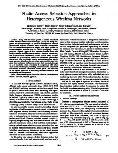
Introduction The Internet was originally designed for communication between stationary hosts performing mostly batch oriented information exchange. However, nowadays mobile hosts and realtime applications have become an integral part of the Internet and the World Wide Web. In parallel, a paradigm shift will soon happen on the telecommunications arena where telephony services until recently have been delivered through dedicated nodes in a specialized circuit switched domain. With the advent of the LTE networks, this will not be the case any longer since LTE has embraced a sole packet domain architecture solution. Yet another important trend is the move of end-user communication services to the World Wide Web. However, until just recently, solutions required users to install third party plug-ins in order to enhance features of existing web browsers. To overcome this problem a standardization effort aiming to improve web browsers’ realtime capabilities was launched by the two main Internet bodies, the Internet Engineering Task Force (IETF) and the World Wide Web Consortium (W3C). The two bodies work closely together where the IETF is currently developing the Real Time Communication in WEB-browsers (RTCWeb) [1] protocols, while the W3C has taken on the responsibility to develop the WebRTC [2] API. The ultimate goal is to provide an infrastructure for developers to deploy realtime communication applications on the web. The WebRTC end RTCWeb architecture is shown in Figure 1.
Fig. 1
The WebRTC and RTCWeb architecture
As mentioned, a WebRTC and RTCWeb provide means for the developer to establish realtime communication sessions directly between web browsers. RTCWeb has, other than handling communication negotiation, several desirable properties to enhance real-time communication sessions on the web. It also aims at coexistence with TCP and, therefore, deals with the TFRC (TCP Friendly Rate Control) [3] protocol. The overall idea is not to use too much capacity while WebRTC applications try to provide the best QoE. The modules included contain minimalistic media components, like the codec itself, an Acoustic Echo Canceller (AEC), a jitter buffer, audio/video modules, functionality for encryption/integrity protection of media, as well as implementation of the Real Time Transport Protocol (RTP) and the RTP Control Protocol (RTCP) [4]. 2
Realtime communication including interactive audio and video applications has always been sensitive with tight timing limitations to packet delay and jitter and in some cases very limited tolerance for packet loss. On the contrary, some applications can tolerate occasional packet loss. One obvious and quite straightforward solution would be to increase the link-rate and capacity of network components in order to accommodate more users and realtime communication applications. However, it would not be a long-term solution due to the rapid increase of subscribers and the increasing demands from them. Also, the network environment in wireless access networks is much more complicated compared to fixed access networks since there is a shared channel used by all users simultaneously. Moreover, users may be roaming from one cell to another the number of mobile users in a cell dynamically changes triggering varying channel capacities. Thus, the wireless communication channel might become a bottleneck at any time and there can easily be high delays in the wireless link, which triggers packet drops and/or increased packet delays and jitter. Hence, providing the required constant level of Quality of Service (QoS) parameters in terms of packet delay, end-to-end delay, network throughput, available bandwidth, packet loss rates, and jitter for multimedia applications is extremely challenging in wireless network environments compared to wired networks. To prevent excessive delays and packet losses in the network, queues need to be kept as short as possible. In order to provide the required level of Quality of Experience (QoE) a congestion avoidance mechanism with a rate adaptation model implemented at the end-systems is hence necessary. For the case of realtime video sessions, there are several rate adaptation techniques that have been proposed including sender-side rate adaptation, receiver side rate adaptation, intermediate node dependent rate adaptation, and both sender and receiver side rate adaptation. We believe that adapting the rate by estimating the congestion occurrence is the most efficient way rather than arranging the rate after severe congestion has occurred and the clients already experienced a lower service quality. This paper proposes and evaluates a congestion avoidance mechanism and a rate adaptation model for WebRTC interactive video sessions in LTE networks where the model is based on realtime available bandwidth estimation and measurements. The rest of the paper is structured in the following way: Section 2 provides related work, while Section 3 describes the implementation of our proposed solution, as well as the Google Congestion Control Algorithm [5], which we have used as a basis for our work. Section 4 describes simulation scenarios and presents the results, while Sections 5 concludes the work, and Section 6, finally, discusses the results and points out future work. 2
Related Work Ho et al. [6] expressed the rapidly expanding demand of real time audio– video stream applications, which do not share the available bandwidth with TCP applications. They present a simulation study of a new loss rate calculating model, which reflects the network state as change of weights in order to provide fairness by adapting the rate. Chowdhury et al. [7] evaluated performance of DCCP by comparing TCP, CCDI2, and CCDI3 of DCCP based on throughput for video/audio applications, which have fixed sending bit rates. Lai et al. [8] also compared DCCP with the TCP congestion control mechanism and eventually the results show that DCCP could achieve TCP’s fairness. Futemma et al. [9] described a middleware 3
where the TFRC-based rate control algorithm was adapted to be used with JPEG 2000 real time video streaming and relies on a loss prediction model. Khanloo et al. [10] observed TFRC over wireless networks. Gevros et al. [11] argued that without any discrimination and any delivery guarantee, all packets are treated the same on the Internet. Satoh et al. [12] proposed a scheme for estimating available bandwidth in simultaneous multiple pair communications, which they called a simultaneous available bandwidth. Gupta et al. [13] presented an experimental comparison of bandwidth estimation tools for wireless networks. Manvi et al. [14] remarked the importance of bandwidth allocation algorithms. Sahasrabudhe et al. [15] presented a bandwidth allocation mechanism to be placed at the base station. This model turned out very well for dynamic measurements and estimation. Bergfeldt [16] provided, in a pioneering manner, the BART tool, estimating instant available bandwidth by actively probing the real time measurement with the dynamic stochastic Kalman Filtering Model. Sarker [17] studied an adaptive mechanism for realtime video in IMS telephony in LTE networks, which relies on ECN notification. Regarding all experimental research, addressed above, it is evident that during a real time interactive video/audio session, estimating available bandwidth and making rate adaptation is vital and provides proved advantages in terms of mitigating the delay and jitter by avoiding congestion collapse. 3
Proposed Solution In order to deal with the bottleneck problem and optimize performance of WebRTC video sessions, this paper proposes a congestion avoidance mechanism and a rate adaptation model, which provides a fair available bandwidth allocation for WebRTC applications, based on real time available bandwidth estimation and measurements over LTE networks. The Google Congestion Control Algorithm’s [5] behavior was used for bandwidth estimation. The proposed congestion avoidance mechanism and rate adaptation model uses two different available bandwidth capacity estimation algorithms in tandem. The first one is the Kalman filtering algorithm that is used to compute states of available bandwidth capacity, ”Under-Using” and “Over-Using”, based on video frame delays as described in the Google Congestion Control Algorithm InternetDraft [5]. The other is the TFRC (TCP Friendly rate control) [3] algorithm, which calculates available bandwidth capacity, based on packet loss rates. TFRC is employed as a post available bandwidth capacity estimation technique to provide fairness between TCP and the real time interactive video traffic flows. The proposed solution consists of two major mechanisms: the first one is a sender control mechanism, running on RTP sender side (terminal side), the other one is a receiver control mechanism and that is placed at the RTP receiver side (network side) as shown in Figure 2.
Fig. 2
Illustration of our WebRTC rate adaptation black box model
4
Sender’s media codec compresses the collected data, from a mic/web-cam, in order to digitize and transmit the media as a sequence of bits based on the bandwidth control mechanism. The sender transmits an RTP stream over the network to the RTP receiver. The incoming RTP stream consists of RTP packets, where the packets contain audio/video frames or both as mixed media. Also, each RTP packet has a timestamp and transmission time offset to provide sender time information to the receiver. When a receiver is receiving an RTP media stream, the receiver stores the arrival time, regenerates the media streams in order to send it to its recipients. Both sides send acknowledgement as follows: RTP sender’s RTCP sender transmits sender reports while RTP receiver’s RTCP sender sends receiver or sender reports and TMMBR/REMB (Temporary Maximum Media Bit Rate/Receiver Estimated Maximum Bitrate) messages to sender side control. A receiver of media also sends RTCP sender reports when the communication is bidirectional. Furthermore, the sender side control mechanism computes a sending bit rate based on the received information. The receiver side control mechanism also considers its received info. The packet arrival time information is used to determine when it needs to send the TMMBR/REM messages. 3.1
Network Parameters and Terms Packet delay, packet loss and network throughput are significantly important parameters to evaluate network performance and they are defined below. A. Packet Delay When packet traverses from one end system to another end system, it suffers from various types of delays: processing delay, transmission delay, propagation delay and queuing delay. Processing Delay ( D p ) is the time, which is required to scan IP packets’ headers and to determine where to forward the packet. There might be other factors, which increase the processing delay, for instance, bit-level errors. Transmission Delay ( Dt ) is the time to push the whole packet into the link
Propagation Delay ( D pr ) is the time which is needed for the packet transmission, from beginning of the link until the packets reaches a router Queuing Delay ( Dq ) occurs, if the link is busy and there are other packets being transmitted. The waiting time depends on the number of packets which are queued to be transmitted. Traffic intensity y has been used to predict the extent of queuing delays. If one IP packet arrives to a router in the time that it can be handled by the router, then the traffic intensity will be close to zero and the outgoing queue will be empty and queuing delays will be wiped out. However, if the packets arrive periodically in bursts, then the traffic intensity will be close to 1, which means that the packet will experience higher queuing delays. B. End-to-End Delay End to end delays can be mathematically defined as follows: if (N-1) routers are deployed on the path from the source and the destination end systems with an assumption, Dend toend (end to end delay) can be simply defined as:
Dendtoend N ( Dpr ( L / R) Dp )
(3.1)
5
where the processing delay ( D pr ) is the same in each router and the hosts the transmission rate for each router and the host is L/R bits/sec, L is the standard packet size, R is the rate and the propagation delay ( D p ), which is the same in each link: For voice applications, humans do not perceive smaller than 150 milliseconds delays and up to 400 milliseconds can be acceptable. As a consequence packets may be dropped in queues, if they are delayed for more than such a given time span. C. Network Throughput There are two types of network throughput: One is instantaneous throughput and the other is average throughput. Instantaneous throughput is the rate of data delivered to the receiver during a time interval. Average throughput is, considering a P2P (point-to-point) communication, sending V bits and delivering it to the receiver takes t seconds, V/t bits/sec. A link j in a network path has a certain throughput capacity Cj, i.e. the amount of bits successfully transmitted over the link per time unit. The traffic intensity over link j is represented by Xj, where: 1 X j j (3.2) t Here, j is the amount of cross-traffic carried off at t time interval over the link j. Note that bit-error probability is typically very low over wired links and the throughput more or less corresponds to the data rate and usually does not change over a wired path. C henceforth can be defined as equal to the data rate. On the other hand, due to fluctuating radio signal strength and other radio channel conditions, throughput capacity on wireless links is often less than the data rate. D. Available Bandwidth and Congestion The bandwidth term refers to the maximum communication channel capacity. When the bandwidth is sufficient, packet delay and jitter network parameters are very low and interactive media applications work quite well in terms of user satisfaction. The time-varying available bandwidth of link j is defined as:
Bj C j X j (3.3) The link along the path that has the smallest value of available bandwidth is called the bottleneck link and it designates the available bandwidth of the entire path. Therefore, the available bandwidth can be expressed as the minimum available bandwidth for all links j along the path from sender to receiver: B min (C j X j ) j
(3.4)
The capacity of bottleneck may lead to excessive delay, packet loss and jitter and called congestion. The available-bandwidth should be seen as an approximation of the possible achievable throughput from end to end sender to the receiver and not a measurement or estimate of the unutilized capacity. The capability of measuring available bandwidth is also significantly important in order to provide accurate results and it is useful in several contexts, e.g. network monitoring. Furthermore, 6
there are various available bandwidth estimation techniques e.g. passive monitoring of available bandwidth and in manner of mathematical models Moreover, since Internet is accessible through multiple interfaces such as WiFi, LTE, etc., correct bandwidth estimation in areas with overlapping wireless access networks coverage has also become vital to provide seamless mobile services providing QoS-guaranteed real-time multimedia applications and in manner of mathematical models. Moreover, since Internet is accessible through multiple interfaces such as WiFi, LTE, etc., correct bandwidth estimation in areas with overlapping wireless access networks coverage has also become vital to provide seamless mobile services providing QoS-guaranteed real-time multimedia applications. E. Packet Loss and Queue Management When a queue is close to getting full or when packets are delayed too long, packets might be dropped due to queue management; the exact behavior depends on the type of the queue with the tail-drop queue being the simplest. Note that the output queuing capacity explicitly depends on the configuration of the router, which might be costly. As mentioned above, a packet arriving might overflow, that is called packet lost or drop, when it is encountered with a full outgoing queue. For instance, if we consider a UDP datagram which is sent by the sender, while it is traversing, passes through the queues at the routers to reach its target destination. If there is excessive delay, long buffering in the routers from sender to receiver, the IP packets might be discarded and never reach its receiver and that is called packet loss. Also, it is evident that the fraction of packet loss will be increased in parallel with the traffic intensity. There are some developed techniques to deal with packet loss. For instance RFC 3290 defines DiffServ functional data path elements and algorithmic droppers, queues and schedulers in the ingress router, Queue management techniques helps to fairly share the outgoing link, and to prevent unnecessary transmission and to provide efficient queuing at the data link layer (layer-2), IP packet scheduling model based on First-In-First-Out (FIFO), a scheduling method that controls each flow in a system with QoS control jointly using Weighted Fair Queuing (WFQ) and dropping packets. WFQ is used at the output port and is considered as important as enough memory in the input port of a router in order to buffer incoming packets. Moreover, dropping packets, in some cases, might be advantageous rather than increasing buffer size. Furthermore, the gateway can itself figure out the optimal action from set of actions by using a Random Early Detection (RED) algorithm and AQM decreases the packet loss. RED arranges the length of the output queue by dropping packets if the average length of the queue is higher than a threshold, which is calculated by a stochastic function and queue length. Additionally note that the queue management algorithms also indicate congestion to end systems. F. Jitter Irregular time periods of delays and high packet loss fluctuate the inter-arrival time of each of the packets and that is called jitter. Note that jitter can be decreased by sorting out the received packets based on the information which is carried in the IP headers such as sequence numbers and timestamps. 3.2
Receiver Side Control Models The receiver side control model is built upon three different parts: an arrival-time filter, an over-use detector, and a remote rate control mechanism. The arrival-time filter is used as described by the Google Congestion Control Algorithm 7
[5]. For the over-use detector and the remote control mechanism, our model relies on a modified version of the Google Congestion Control Algorithm [5] in order to decrease the complexity of the algorithm. The arrival-time filter is described in Sections 3.2A and 3.2B below. The over-use detector is described in Section 3.2C, while Section 3.2D describes calculation of the packet loss event rate ‘p’ value, which is taken into consideration by the sender while it regulates its video output bitrate. This is called the remote rate control mechanism. A. Receiver-Side Arrival Time Model The instant traffic in computer networks can be modeled as a stochastic process. Therefore, adaptive filtering is required in order to continuously update the network parameters based on the timing and received frames’ features. Frame size, received time and time stamps are examples of that. The packets have the same time stamps, if they are corresponding to the same frame, and any packet loss is avoided at this stage. The sender marks each frame while being transmitted with tsent as well as the receiver marks it with treceived when it is delivered, where i { | 1...n} . The sent-time interval Δtsent(i) between two consecutive frames i+1 and i is calculated as: Δtsent(i) = tsent(i + 1) tsent(i) (3.5) The same is done for Δtreceived. Furthermore, encoded frames of a regular video codec usually are the same size. However, there might be some I frames (key frames) that may be significantly larger, and they need more time to traverse the link. Hence, large frames may cause congestion and higher delays. Therefore, it is evident that a frame’s delay is relative and depends on other frames’ size, which also was taken into account during development of the delay based congestion control algorithm as defined by Google [5]. Hence, the inter-arrival time tinter-arrival(i) is defined as following: tinter-arrival(i) = Δtreceived(i) Δtsent(i) (3.6) On the other hand, frame i’s transmission time is represented by Tsent and that can be formulated as follows:
Tsent (i )
L(i ) C (i )
(3.7)
where C(i) is the capacity (as defined in Section 3.1C) and L is frame i’s size. Furthermore, if we assume that C(i) is the capacity and W(i) is a sample of W (stochastic process function of the capacity), the inter-arrival time model can be defined as follows: -
()
()
(
)
()
()
(3.8)
It should be noted that the noise corresponds to the jitter and other delay effects, which cannot be captured by the inter-arrival time model. The White Gaussian process function W(i) is increased, and for the case of congestion in the communication channel, it will be zero correspondingly with degradation of bandwidth usage. Breaking out the mean m(i) from W(i) to make the process zero means: -
()
()
()
()
(3.9) 8
The usage of current bandwidth C(i) and the available bandwidth capacity m(i) need to be estimated for each next frame’s transmission process respectively. This is done by calculating the current available bandwidth based on the experience that we obtained from the latest received frame delivery to the receiver side. Furthermore, V(i) represents noise variance. B. Receiver-Side Arrival Time Filter Model The Google Congestion Control Algorithm [5] uses Kalman filtering to observe how the realtime interactive system state is related. This is done using repeated measurements of some quantity of the network. The algorithm also filters how the usage of bandwidth evolves during the realtime interactive session. After simulating the algorithm, we discovered that “Normal” is a redundant state, and hence only use “Under-using” and “Over-using”. We have shown how tinter-arrival can be calculated and ΔframeSize is calculated as the difference in size between two consecutive frames. These network parameters can be gathered by a recursive stochastic Kalman network filtering algorithm even though video frames are fragmented. If the frame size is greater than the Maximum Transmission Unit (MTU) the frame will be fragmented into multiple IP packets, which will all have the same time stamp. The Kalman filtering model is an adaptive filter that continuously updates the estimates of network parameters based on received frames, the timing and linear equation of the previous estimation and new measurements. Afterwards, the Kalman filtering model updates the estimation of the system state based on the previous measurement. The network system state x at time k can be defined as follows:
m( k ) xk 1 / C (k )
(3.10)
The dynamic network system can be represented in the time domain linear equation:
xk Axk 1 wk 1
(3.11) where the system state model evolves from discrete time k-1 to k. The A2x2 matrix in the equation relates the current state k to the previous time step k-1, in the absence of process noise. Note that A is a dynamic parameter, which might change in each time step. On the other hand, the system measurement model can be defined as follows:
zk H k xk Vk
(3.12) where z represents the measured system quantity and V represents the white Gaussian with variance measurement noise. The average bitrates of received frames has been taken into account as follows: (3.13) H k = éê D frameSize(k) 1 ùú ë û The Kalman filtering algorithm runs the system state estimation part model that is defined as follows: ~
xk Axk 1
(3.14)
where the previous estimation xk-1 has evolved. 9
At the measurement phase the algorithm computes the updated covariance matrix P:
Pk (1 K k H k ) Pk
(3.15)
Pk APk AT Q
(3.16)
and
where the stochastic variation of the noise is represented with Q and Kk represents Kalman gain:
K k Pk H kT ( H k Pk H kT R) 1 Pk H kT Vk1
(3.17)
The Kalman filter formalism is applied with A=I2x2 identity matrix, which is the relative weight of the new measurement at the discrete time of k showing that the predicted evolution of the previous state estimation, which was done at discrete time k-1. The variation of the noise is the evaluation of system weight prediction. The stochastic variation of the measurement noise is represented with V that indicates the evaluation of the system weight measurement. The Kalman gain is related with Q and V, and it increases as either Q increases or V decreases. When realtime video frames are transmitted over the network, all the abovementioned rate control schemes could not work well since they do not adapt to dynamic available bandwidth capacity in the network. Also, other varying conditions, e.g. delay conditions that vary from time to time, might lead to problems. Noise estimation and measurement values are therefore recursively updated using an exponential averaging filter for the estimated variance noise Q and modified for variable sampling rate as follows:
Q (v, i) 2 (1 ) * z (i )
(1 ) f
(3.18)
max
where
f max max{
1 }, j (i k 1), i sent ( j ) sent ( j 1)
(3.19)
j is the highest rate at which frames have been captured since the last captured k video frames. A filter coefficient has been chosen as 0.1,0.001. The noise v(i) should be zero, which means that white Gaussian noise might be less accurate in some circumstances, e.g. when the network throughput is higher than the capacity. Therefore, an additional outliner filter has been used as update mechanism as follows: If z(i) > 3Q, then the filter is updated with 3 Q rather than z(i). In a similar way, Q(i) is chosen as a 2x2 diagonal matrix with main diagonal elements being defined by T 30 (3.20) diag (Q(i)) 1010 102 (1000 * f max ) It is necessary to scale these filter parameters with the frame rate to make the detector respond as quickly at low frame rates as at high frame rates.
C. Receiver-Side Bandwidth-State Detector The set of estimated bandwidth states contains two estimate-bandwidthusing states “Over-Using” and “Under-Using”. Bandwidth state estimation is 10
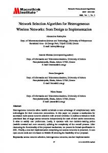
related with time of last estimated available bandwidth using state as well as the number of received large frames, which are triggering the “Over-Using” state indication. The system’s “Under-Using” state means that there are not so many large frames queued in the network path (IP layer) and the queues are being diminished, which is indicating an estimate of available bandwidth capacity is higher than the actual available bandwidth. As shown in Figure 3, video frame delay-based estimate (calculated by the Kalman Filtering Algorithm) is compared with a threshold in order to determine the state. When the estimation is greater than the threshold value, it is considered as an indication of “Over-Using” bandwidth state. Note that, sometimes even if the estimation is greater than the threshold that is not adequate to trigger and send a signal of “Over-Using” estimate to the sender side rate controls’ subsystem. This happens because when the offset estimate is greater than the last update (the offset value of previous state), a certain estimate “Over-Using” state decision will be made and signaled when the over-use has been detected for at least two times. Otherwise, if these conditions are not met, the signal will not be triggered even though “Over-Using” is detected. Similarly, the other estimate-state “Under-Using” is detected, when estimated available bandwidth is smaller than the threshold value. The global system response time is the time from an increase/a decrease that has caused indifferent states until a new bandwidth usage estimate state is detected. A new state means that the new detected state is different than the previous estimated state by the bandwidth-state estimate detection model. When the new estimate state is detected, the noise variance will also be updated, and that is used as a parameter in the Kalman Filtering Algorithm as mentioned in the previous section. Thus, the bandwidth-usage estimated state is an indicator of the video frame delay inflicted by the Kalman filter. Once the estimate of available bandwidth state has changed, the receiver immediately has to transmit the detected state as an RTCP feedback message [7] to the sender in order to inform the sender-side rate control model. Note that receiver’s each transmitted feedback message also contains a packet loss event rate, which is described in the next section. The receiver can basically transmit the report whenever the state is changed. However, the RTCP feedback report transmission time frequency has a timelimitation on how fast the sender can regulate by decreasing/increasing the interactive video output bit rate. This is because it is evident that sending lots of feedback messages for the same estimate rate level means sending no new information leading to a waste of network resources, especially the bandwidth. On the other hand, transmitting few feedback messages might also result in a failure to react in a timely manner. The feedback messages can also be lost in the case of severe congestion on the feedback channel as explained in the background section. Feedback messages should be sent using a "heartbeat" schedule allowing the sender side control to react to missing feedback messages by reducing its send rate. They should also be sent, whenever the state is changed, without waiting for the heartbeat time, up to some limited upper bound of the send rate. In our simulation model, an ideal feedback channel is used in order to isolate the achievement of the ideal rate adaptation model from RTCP’s negative effects, whenever the estimated rate level has changed in order to assure the systems’ maximum working efficiency.
11
Fig. 3
Bandwidth-Usage-State Detector Algorithm Flow Chart
D. Receiver-Side Packet Loss Event Rate ‘p’ In order to compete fairly with TCP flows, the WebRTC real time video receiver calculates the packet lost event rate. However, the Google Congestion Control Algorithm [5] does not include any implementation details of the calculation of the ‘p’ value. As specified in RFC 5348 [3], the receiver assumes that the sequence number is incremented by one for each packet that is sent and keeps track of arriving packets based on the sequence number to obtain some information (e.g. sequence number, packet size, time stamp, etc.). The receiver increases the number of received packets for each received packet and compares the number of received packets with the acquired sequence number of the last received packet. If the sequence number of the last received packet is not equal to the number of received packets that means a packet has been lost just before the receiver received the last packet. When a lost packet has been detected, the lost packets’ nominal arrival time, Tlost, is calculated at the receiver side:
TLost
TBefore (TAfter TBefore ).(S Lost S Before ) S After S Before
(3.21)
where Slost is the sequence number of lost packet, TBefore is the reception time of the received packet just before the lost packet occurred, SBefore is sequence 12
number of received packet just before the lost packet occurred. TAfter and SAfter are respectively reception and sequence numbers of the received packet right after the packet is lost. If we consider that there are two determined lost packets. SLost_A is the sequence number of the first determined lost packet A and B being the next determined lost packet right after A is lost, has sequence number SLost_B. If we assume that TLost_A and TLost_B are the nominal delivery times of A and B respectively and if TLost_A + R > TLost_B in that case packet loss B is part of the last loss event, it is avoided. Otherwise B is the first lost packet in a new loss event. If SLost_B is the first packet in a new loss event, then the number of packets in loss interval A is given by
I Lost S Lost _ B S Lost _ A
(3.22) The average loss interval is smoothed in a filter, which weights the n most recent loss event intervals. The number of loss interval is n which is equal to 8 as recommended in RFC 5348, n should not be greater than 8 for competing with TCP in the global internet. The values of weights are given by the following set:
W = {0.1, 0.1, 0.1, 0.1, 0.8, 0.6, 0.4, 0.2}
(3.23)
If ILost_0 to ILost_7 are the most recent 8 packet loss intervals, the average loss event rate p can be calculated as follows:
p
1
(3.24)
I mean
where the average loss rate is: 7
I mean
I n 0 7
n
w n0
(3.25) n
In reality there might be some issues while receiving packets such as IP packets might not be delivered in order to the target receiver or the sequence number might be wrapped between Si-1 and Si+1, etc. This may happen for instance when packets take different paths as a result of load balancing in the network. How to handle the given issues are explained in RFC 5348 [3]. These issues are already avoided in the network simulation. Therefore, they are not implemented in our case. The sender uses the p value when calculating the TFRC network throughput value whenever a new feedback message is received. 3.3
Sender Side Control Models The sender-side control model consists of two major mechanisms: TFRC Bandwidth Estimation model and Sender-Side Real Time Rate Control Mechanism, which are descried below. A. TFRC Bandwidth Estimation Model Recall that the congestion control mechanism is a requirement for all applications that wish to share the network resources as described in RFC 2914 [18]. Therefore, RTCWeb also aims to be reasonably fair, when competing for bandwidth with others, like TCP flows, by avoiding unnecessary fluctuations in the sending rate. 13
The RTP packet-loss based TCP throughput equation has been considered, while the sender-side real time video model is throttling the real time video outputrate as a control formula of receivers’ feedback as specified at TFRC. TFRC is another type of available bandwidth estimation algorithm, which relies on the p value (the packet loss-rate).
TTFRC
s 2p 3p RTT t RTO (3 ) p(1 32 p 2 ) 3 8
(3.26)
where s represents the average size of received packet size per second, RTT is round trip time and tRTO is the value of the retransmission timer. Note that the equation of TTFRC does not represent the actual WebRTC real time video output rate but it represents an upper bound for it. RFC 5348 [3] also briefly explains the calculation of all given parameters. The variation of TFRC is significantly lower than the variation of TCPthroughput, which provides a more suitable mechanism for real time interactive media where throttling sending output rate is crucial. This implementation is also designed with a failure tolerance mechanism. As a failure reaction, if the sender does not receive estimated available bandwidth state feedback (report) within a certain time period that is two times longer than the length of maximum interval, the real time video output-rate scheduler algorithm is designed to make an assumption. It then assumes that there is congestion, which occurred on the feedback channel and that the feedback reports were lost. In that case, the TFRC value will immediately be halved. It should be noted that for the ideal feedback channel case, this failure mechanism is not implemented. B. Sender-Side Real Time Rate Control Model The rate control model at the sender side was developed to determine the video output-bit rate by considering both the received delay-based state of available bandwidth from the real time video receiver-side and sender side TTFRC estimate bitrate value which is calculated based on receiver-side packet loss rate. The sender side real time interactive video rate control algorithm runs whenever a receiver’s feedback report arrives to the sender as shown in Figure 4. That occurs no more often than at minimum round trip time, and no less often than at a maximum interval.
14
Fig. 4
Sender Side rate control algorithm flow chart
The model increases the real time video output-rate, when the sender has received the “Under-Using” state as long as the TTFRC estimate bitrate is greater than the sender’s actual bitrate. Also, the model decreases the real time video output-rate when the received bandwidth state report is “Over-Using” or if the sender’s actual bitrate value is greater than the calculated TTFRC estimate bitrate. The adaptive real time video output bitrate level consists of 6 different values from 1 to 6, which are corresponding to the real time interactive video output-bit rate values; 200 kbps, 300 kbps, 400 kbps, 500 kbps, 800 kbps and 1000 kbps. If the level is 3, for instance, that is corresponding with the third video output-bit rate, which is 400 kbps and that means that the sender’s actual video transmission bitrate is 400 kbps. Assuming that the TTFRC estimate bitrate is greater than sender’s actual video bitrate and the adaptive real time video output rate level is 3, if the received feedback available bandwidth state is “Under-Using” the sender bitrate will be increased to 4. On the other hand, if assuming that the calculated TTFRC estimate is lower than the sender’s output bitrate regardless the received state is “Over-Using” or not, the sender side rate control model decreases the bitrate level to 2. If the received feedback message conveyed an “Over-Using” state regardless of the calculated TTFRC estimate bitrate, the sender side rate control model reduces the sender’s output bitrate. Finally, the actual video transmission bitrate will also be increased or decreased one step up or several steps down at a time in parallel with the level of video output rate. Whenever the received state is “Under-Using”, the adaptive real time video output rate level will increase the video rate level, as long as the actual bitrate value is lower than the TTFRC estimate value. By working that way, the model ensures that the actual estimated rate is never higher than the TTFRC estimate. When “Under-Using” state is received and if the TTFRC value is not greater than the actual bitrate, the system will not increase the actual bitrate. Thus, the TTFRC value plays a vital role as an upper bound for the actual bitrate. If the amount of the packet loss over the transmission channel is low and the received feedback message is “Over-Using”, the sender does not increase its bit rate, because when the “Over-Using” state occurs it is evident that the packet loss value definitely will be increased after a while. This is because of “Over-Using” state means that the video frame delay is increased because the queues in the network became longer and that causes AQM to drop packets (where AQM is supported). Hence, soon the system TTFRC parameters will drop down the bitrate. However, even if the detected state of the Kalman Filtering model is “Over-Using” and the TTFRC estimate bitrate does not decrease the network throughput, that means that the packet losses are probably not related to shared-link “Over-Using” state. Therefore the system will still decrease the bitrate. By doing that, TFRC makes rate adaptation to work better. Note that the rate control subsystem makes the assumption that at the beginning of the WebRTC real time interactive sessions, the bandwidth state is in an “Under-Using” state. It then initiates the video-output bitrate from the first 200 kpbs. The next step is to slightly smooth the video output rate level step by step, as long as the TTFRC estimate value is greater than the actual bitrate, until the system has reached the instant maximum capacity, an “Over-Using” state message is received or the TTFRC estimate is decreased. 15
If the sender side real time video rate controller does not receive any signal recall that TTFRC will be halved and the module assumes that the available bandwidth state is not changed since the last reduction or increment of the output rate. Then it keeps increasing or decreasing based on the intention of the last received state, as long as the halved TTFRC parameter allows. Note than when using an ideal channel, due to all feedback messages being received, this failure tolerance mechanism is not implemented. On the other hand, in some cases the assumption, of course, might be wrong and the state might be already “Over-Using” at the beginning of the WebRTC session; then the TTFRC estimate will also be low. Therefore, the sender will keep the lowest bitrate but always try to increase it as soon as possible. The rate adaptation model reduces the video frame delay, whether AQM is supported or not, Related with decreased video frame delay, the algorithm will increase the user satisfaction level as targeted, another expected effect is that it will decrease the senders’ out bitrate when in the “Over-Using” state, or will increase the bitrate, when in the “Under-Using” state as long as the TTFRC estimated value is greater than the actual bitrate. In the rate adaptation model, the TTFRC available bandwidth estimate is computed for each received p value within RTCP packets and the updated TTFRC value is considered for each transmitted video frame. Furthermore, the Google Congestion Control Algorithm [5] does not specify the p value calculation. At these points, our proposed solution slightly differs from it. 4
Simulations and Results This section presents the simulations performed, where the new generation browsers’ embedded WebRTC mechanism is extended with our proposed congestion avoidance mechanism and rate adaptation model. The simulations observe a set of the network system parameters, including video frame delay, packet loss rate (%), and average bit rate of sender’s real time video. Measurements and evaluations have been carried out using a Java based system simulator and the Matlab tool. In order to observe the performance of the presented rate adaptation model, the number of active users was varied in three different simulation scenarios, namely single Video traffic, mixed Video-VoIP traffic, and mixed Video-VoIP-Web traffic. The traffic scenarios have been simulated where Active Queue Management (AQM) was turned on and off, while the data traffic was transmitted over LTE interface. Also, uplink and downlink scenarios were simulated separately in order to decrease the number of dependences. 4.1
Simulation Environment A professional Java based network system simulator has been used in this study, which is able to perform simulation scenarios over various wireless access network topologies as well as different network protocols. In this study, the 3GPP LTE typical-urban-topology area network model with seven sites and a total of 21 hexagonal cells (3 cells per site) was used. The simulation environment is able to generate users at specific times with certain intensity (a number of generated users per second) as well as with specific traffic types, e.g. video, voice, or both voice-video, etc. The most important feature of the simulator is that it allows us to log any information and parameter values for later post processing. Therefore, a number of different intensities have been used to be able to provide a certain number of users {1, 2, 3, 5, 7, 10} users per cell and each user has video or video-voice or video– 16
voice-web traffic flows. Also the initial number of active users is zero for all scenarios and this number of active users was slightly increased with a certain number called intensity. Due to the instantly varying number of users per cell, the network throughput changes dynamically during the simulation time. The active users are randomly distributed over the simulation area; therefore, the given number of users per cell is an average over all cells (total number of users is divided by number of cells, which is 21). That means there might be some cells, which have higher or less number of users connected to it. Additionally, we assumed that when the users are involved with the simulation scenario the communication channel is already established; by doing that the session set up failure problem is avoided. The time duration of the experimental simulation scenarios was set to 181 seconds, where each WebRTC real time client had a 60 seconds lifetime. All simulation scenarios have been performed with the same time duration of interactive video/audio, which is equal to the WebRTC clients’ lifetime. Therefore, the session is initiated as a video or video-audio chat session when the users are activated. The session is terminated when the user has left the floor (terminated the session). Also, we considered that, in some scenarios, during the interactive session the clients might be surfing the web as well. The WebRTC interactive video traffic model was used to generate real-time client’s video traffic with various video bitrates: 200, 300, 400, 500, 800, and 1000 kbps using the same video codec H.264. The simulation model also enabled us to trace each video frame and RTP packet (sent over UDP) to get information about the packet size, sequence number, frame received/sent time, etc. in a realistic way. Note that, some parts of our model were replaced at the application layer and transport layer in order to get some statistics and information from the RTP packets as shown in Figure 5.
Fig. 5
Protocol Chains of the LTE Simulation Model
The VoIP session starts at the same time as the interactive video session and the conversation continues during the interactive video chat session between two users. In order to observe the impact of TCP traffic on WebRTC interactive sessions, each user might also surf the web during a video chat session. Therefore a web surfing traffic model was configured, where each user has an HTTP traffic flow, and aims to download 100 KB sized web pages 20 times from www.amazon.com. The client also waits between downloads, reads the page, during a random time length, which is from 2 seconds up to 20 seconds. Additionally, the users are roaming around with 30 km/h speed, which should also be taken into account, because, there will be more frequent handovers and faster changing channel quality than if the users move around more slowly.
17
4.2 Results A. Single User Traffic Results Using the given sample user figures, we can observe the results of how rate adaptation has been carried out based on receiver side Kalman filtering as well as sender side TTFRC estimated bitrate. Some randomly selected users’ simulation results have been examined. The first three plots given by Figure 6 shows the receiver’s traffic experience: the first graphs shows that the video frame delay that is experienced by the receiver and the second and third graphs indicates Kalman filtering detection. Furthermore, the fourth plot presented in Figure 6 shows a sample user’s (the sender-side) traced traffic flow, which has a single video traffic, downlink, where AQM is not supported and number of deployed users is 3 per cell. The user has a lifetime between 60 seconds and 120 seconds in the simulation time (represented by the x-axis). The implementation of our model starts increasing the bitrate step by step at the beginning of the WebRTC session due to TTFRC network bitrate estimation being greater than the sender’s actual bitrate and receiver side using-state indication is not “Over-Using”. We can observe that at t=70 seconds the video frame delay increases up to 0.5 second, which is detected at the receiver by the Kalman Filtering algorithm and indicated to the sender as a “Over-Using” state with a RTCP feedback message. When the feedback message is delivered to the sender, at the sender side the rate adaptation decreases the video traffic bitrate from 1000 kbps to 800 kpbs. When the queues are shortened in the network, “Over-Using” state indication has been changed to “Under-Using” state and the sender increased its output video bitrate one step up to 1000 kpbs. After a while we also observed that with the decreased TTFRC estimate the sender’s video bitrate has been decreased one step down to 800 kpbs and related with maintained and decreased TTFRC value it drops to 600 kbps even though the indication state is not “Over-using”. Additionally, we can see that the TTFRC estimate is fluctuating and pushes down the video bitrate even if there is no congestion at last quarter of the user’s lifetime. DL,S-B-Video-AQM-F
Video Frame Delay 1
Video Frame Delay 0.5
0 60
70
80
90
100
110
120
User Life Time [s]
Detect, Threshold 0.1
abs(T) threshold
0.05
0 60
70
80
90
100
110
120
Detect,Over-Using Counter 10
overUseCounter hypo
5 0 60
70
80
90
100
110
120
110
120
Bitrates [Kbps]
1000
0 60
Fig. 6
curr bitrate
500
nom bitrate TFRCrateValue 70
80
90
100
A sample User-DL, Single Video Traffic where AQM is Turned OFF
18
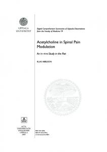
B. Single Video Traffic Results In order to clarify attributes of the network parameters and the performance of our proposed solution, the system simulation has been run with a fixed 1000 kbps average video bitrate for downlink and uplink single interactive video traffic scenarios (with the our model turned OFF). The reference simulation results show that when the number of users is increased in one cell, the available bandwidth per user is slightly decreased and triggered the bottleneck. Therefore, the queues became longer in the network. Where AQM is turned ON, AQM dropped even more packets. Eventually, excessive video frame delays occurred where AQM was not turned OFF and the packet loss rate increased systems at the end, where AQM was turned ON. The reference average video delay results show that the system will be useless, when the numbers of active users are more than one user per cell at uplink and 3 users per cell at downlink respectively, due to the video frame delay is higher than 1 second, where AQM is turned OFF. On the other hand, the simulation results of the single video traffic scenario with the rate adaptation model show that QoE is good enough up to 7 users/cell even when AQM is turned OFF. The results of the single interactive video scenario are identical to the results with a mixed Video-VoIP scenario in all four cases at uplink and downlink. Therefore, those results are not given in this paper. This would mean that transmitting additional real time voice frames along and through the communication path does not overwhelm the network. C. Downlink-Mixed Video-VoIP Traffic Results To simulate a WebRTC video chat session, as mentioned above, this scenario contains each user to have two traffic flows, namely mixed Video and VOIP respectively. In this case it is worth to remark that the our model is turned ON and arranges the video bitrate in order to adapt dynamically to available bandwidth capacity. The results of mixed video-VoIP traffic scenarios are, for both cases, likely single video traffic transmission, 100% of the active users have experienced the average video frame delay less than 0.2 seconds regardless of whether AQM is supported or not. Moreover, the results indicate that 95% of deployed users have experienced the video frame delays less than 0.2 seconds. For both cases, the packet loss rates are less than 1% for 90% percent of active deployed users. One may also observe that packet loss rates are a bit higher when AQM is turned ON. As a consequence, regarding high capacity of LTE downlink, the bottleneck problem has not been observed in this scenario. D. Downlink-Mixed Video-VoIP Web Traffic One of the most recent discussions in the IETF is how WebRTC real time traffic flows are affected by TCP flows and how to provide fairness between the TCP and RTP flows [21]. In this scenario, to be able to examine the impacts from TCP flows on real time media during real time interactive video chat sessions, the client also surfs the web as described above. D.1 Sender’s Average Video Bitrate Regarding the described scenario of surfing the web during the real time WebRTC video chat session, it is obvious that the TCP traffic had impact on the real time media transaction as seen in Figure 7, which represent CDF plots of average bitrate of mixed video-VoIP and web traffic scenarios. 19
One has to keep in mind that the simulation results from the Video-VoIP scenario with 10 users/cell and 7 users/cell show that 30% and 100% of the users respectively used an average bitrate more than 200 kbps, when AQM was turned ON and OFF respectively. The results of the mixed-VoIP and web traffic scenario and the Video–VoIP scenario are different, when the network is loaded with 7 and 10 users/cell: 30% and 100% of loaded users respectively were locked at 200 kbps, when AQM is turned ON. The reasons for sending the lowest bitrate by senders are the following: the rate adaption regulates the bandwidth based on the receivers’ feedback messages at the sender’s side. Therefore, the available bandwidth state is “Over-Using” for most of the users who are locked at the lowest bitrate level. On the other hand, TCP traffic is the major reason for the long queues which usually increases packet loss rate at the network which decreases the TTFRC value of the WebRTC real time video senders and thus the senders’ average bitrates. Additionally, when the AQM is turned ON it is evident that the number of lost packets will be higher and packet loss rate is higher at the receiver side. Therefore, the received packet loss rate decreases the TTFRC estimate and that pushes down the senders average output video bitrate. DL,S-B-Video-Voip-Web-AQM-T
DL,S-B-Video-Voip-Web-AQM-F
1
1
0.9
0.9
0.8
0.8
0.7
0.7
1 users/cell 2 users/cell 3 users/cell 5 users/cell 7 users/cell 10 users/cell
0.5 0.4 0.3
0.6
CDF
CDF
0.6
0.5
0.3
0.2
0.2
0.1
0.1
0 200
300
400
500 600 700 Average Bitrate [Kbps]
800
900
1000
1 users/cell 2 users/cell 3 users/cell 5 users/cell 7 users/cell 10 users/cell
0.4
0 200
300
400
500 600 700 Average Bitrate [Kbps]
800
900
1000
Fig. 7 a+b Average Bitrate Downlink, Mixed Video-VoIP-Web Traffic, and AQM is Turned ON and OFF respectively
D.2 Video Frame Delay Figure 8 presents CDF plots of the average video frame delay. Notice that, in all cases of the mixed video-VoIP scenario, the average video frame delay was less than 0.3 seconds for all number of deployed users. Where AQM is turned ON, the average delay is still less than 0.3 seconds for all number of deployed users. However, when the system is loaded with 10 users/cell and AQM is turned OFF, the average delay is dramatically increased with higher number of users as a consequence of reaching the maximum capacity of the LTE downlink channel. In that case, there is nothing to do for our model, because TCP traffic is the reason for long queues in the network.
20
DL,S-B-Video-Voip-Web-AQM-T
DL,S-B-Video-Voip-Web-AQM-F
1
1
1 users/cell 2 users/cell 3 users/cell 5 users/cell 7 users/cell 10 users/cell
0.9 0.8 0.7
0.9 0.8 0.7 0.6
CDF
CDF
0.6 0.5
0.5
0.4
0.4
0.3
0.3
0.2
0.2
0.1 0
1 users/cell 2 users/cell 3 users/cell 5 users/cell 7 users/cell 10 users/cell
0.1
0
0.1
0.2
0.3 0.4 0.5 0.6 0.7 Average Video Frame Delay [s]
0.8
0.9
0
1
0
0.1
0.2
0.3 0.4 0.5 0.6 0.7 Average Video Frame Delay [s]
0.8
0.9
1
Fig. 8 a+b Average Video Frame Delay Downlink, Mixed Video-VoIP and Web Traffic. AQM is Turned ON and OFF respectively
Figure 9 shows tail latency, which gives the delay for 95% of the delivered frames to all users. Regarding the tail latency results, 95% of the users have received the video frames with 0.5 seconds delay, where AQM is turned ON. When the system is loaded with 10 users per cell and AQM is turned OFF, 95% of the deployed users’ QoE was not good enough, because they received the frames 1.8 seconds too late, which renders the system useless. DL,S-B-Video-Voip-Web-AQM-T
DL,S-B-Video-Voip-Web-AQM-F
2
2 videodelay 95%
1.8
1.8
1.6
1.6
1.4
1.4
Video Frame Delay [s]
Video Frame Delay [s]
videodelay 95%
1.2 1 0.8 0.6
1.2 1 0.8 0.6
0.4
0.4
0.2
0.2
0
0
1
2
3
4 5 6 Number of Users/cell
7
8
9
10
0
0
1
2
3
4 5 6 Number of Users/cell
7
8
9
10
Fig. 9 a+b Tail Latency Downlink, mixed video–VoIP and web traffic. AQM is turned ON and OFF respectively
D.3 Packet Loss Rate (%) Figure 10 presents the results of packet loss rates for mixed video, VoIP and web traffic, where AQM is turned ON and OFF respectively. The packet loss rates of mixed traffic video and VoIP were 1.5% for both cases. It is quite clear that the presence of TCP flows increased the long queues, which causes the AQM algorithm to drop packets. Eventually the packet loss rate reaches up to 5% when the number of active users is 10 per cell and AQM is turned ON. Furthermore, the packet loss rates were less than 1.5% in the both cases where AQM is turned OFF. This exemplifies the tradeoff between delay and packet loss.
21
DL,S-B-Video-Voip-Web-AQM-T
DL,S-B-Video-Voip-Web-AQM-F
1
1
0.9
0.9
0.8
0.8
0.7
0.7 0.6
CDF
CDF
0.6 1 users/cell 2 users/cell 3 users/cell 5 users/cell 7 users/cell 10 users/cell
0.5 0.4 0.3 0.2
0.5 0.4 0.3 0.2
0.1 0
1 users/cell 2 users/cell 3 users/cell 5 users/cell 7 users/cell 10 users/cell
0.1
0
0.5
1
1.5
2 2.5 3 Packet Loss Rate (%)
3.5
4
4.5
5
0
0
0.5
1
1.5
2 2.5 3 Packet Loss Rate (%)
3.5
4
4.5
5
Fig. 10 a+b Packet Loss Rate (%) Downlink, Mixed Video-VoIP and Web Traffic. AQM is Turned ON and OFF respectively
E. Uplink Mixed Video-VoIP Traffic Results As a consequence of the limited capacity of the LTE uplink channel we observed that in both cases the system is started with a relatively good average bitrate. When the maximum number of active users is deployed, the average bitrate level increased one step up in order to prevent long queues at the network components and keep the video delay as low as possible. Once again, we observed that the results are better when AQM is turned ON, rather than turned OFF. When AQM is turned ON, the average video frame delay is 0.4 seconds. These are the same values as for the uplink-single video transmission case. Where the number of active users is more than 5 while AQM is turned OFF, the value increases to more than 1 second. For the simulation scenarios with 10 active users per cell deployed and with AQM turned ON, the packet loss rates are less than 5% for 90% of the deployed number of users. Furthermore, it is less than 3% for all number of loaded users/cell, which is the same with the results of the single video traffic scenario. The results are quite similar with uplink single video transmission. This is an indication that the delay based rate adaptation algorithms are not that well suited for real time interactive traffic. F. Uplink Mixed Video-VoIP and Web Traffic As mentioned above, TCP flows will be involved in this scenario as additional data traffic together with the pervious scenario with mixed Video-VoIP traffic and AQM being turned ON or OFF. This is done in order to clearly observe the impact of TCP flows on real time interactive media traffic at uplink traffic. F.1 Sender’s Average Video Bitrate Figure 11 shows average bitrates for uplink mixed Video, VoIP, and Web traffic, where AQM is turned ON and OFF. 100% of the active users had the lowest video bitrate when the system was loaded with a more than 5 users/cell. This is corresponding to limited LTE uplink capacity and the impact of TCP traffic on average bitrates for the users who had the lowest average bitrate. This is due to TCP traffic triggered long queues in the network and the video frames delivered lately, which triggered “Over-Using” state and also increased the number of dropped packets subsequently decreased the senders bitrate.
22
UL,S-B-Video-Voip-Web-AQM-F 1
0.9
0.9
0.8
0.8
0.7
0.7
0.6
0.6
CDF
CDF
UL,S-B-Video-Voip-Web-AQM-T 1
0.5 0.4
1 users/cell 2 users/cell 3 users/cell 5 users/cell 7 users/cell 10 users/cell
0.3 0.2 0.1 0 100
200
300
400 500 600 700 Average Bitrate [Kbps]
800
900
0.5 0.4 1 users/cell 2 users/cell 3 users/cell 5 users/cell 7 users/cell 10 users/cell
0.3 0.2 0.1 0 200
1000
300
400
500 600 700 Average Bitrate [Kbps]
800
900
1000
Fig. 11 a+b Average Bitrate Uplink, Mixed Video-VOIP and Web Traffic. AQM is Turned ON and OFF respectively
F.2 Average Video Frame Delay Figure 12 presents results of average video frame delay of uplink mixed video, VoIP, and web traffic, where AQM is turned ON and OFF. When AQM is turned ON, the average video frame delay is less than 0.4 and 0.6 seconds. Also, the results show that when TCP flows are involved, the experienced average video delay is doubled and can be observed it reached 0.6 seconds. Note that, the experienced high delays triggers “Over-Using” state and is one of the reasons for the decreased average video bitrate and increased the packet loss rate. On the other hand, when 10 users are deployed per cell and AQM is turned OFF the system become useless for 99% of the users. Only 30% of the users experienced the delay to be less than 1 second. This is because of the LTE network uplink capacity already having been run out. Henceforth, 10 users per cell is too much for uplink and the average bitrate is hit to the ground per user. The average video delay has also been increased in parallel with the increased active users per cell, which triggered long queues at the network components as well as additional web traffic. Note that the average delay was much lower and the packet loss rate is extremely high when AQM is turned ON. UL,S-B-Video-Voip-Web-AQM-F
UL,S-B-Video-Voip-Web-AQM-T
1
1 1 users/cell 2 users/cell 3 users/cell 5 users/cell 7 users/cell 10 users/cell
0.9 0.8 0.7
0.9 0.8 0.7
CDF
CDF
0.5
0.5
0.4
0.4
0.3
0.3
0.2
0.2
0.1
0.1
0
1 users/cell 2 users/cell 3 users/cell 5 users/cell 7 users/cell 10 users/cell
0.6
0.6
0
0.1
0.2
0.3 0.4 0.5 0.6 0.7 Average Video Frame Delay [s]
0.8
0.9
1
0
0
0.1
0.2
0.3 0.4 0.5 0.6 0.7 Average Video Frame Delay [s]
0.8
0.9
1
Fig. 12 a+b Average Video Frame Delay Uplink, Mixed Video-VoIP and Web Traffic. AQM is Turned ON and OFF respectively
When the system is loaded with the maximum number of users/cell and AQM is turned ON, 95% of the users have experienced video delays less than 0.7 seconds as seen in Figure 13. When AQM is turned OFF the average video delay is more than 2 seconds where 5 users/cell is deployed. Therefore, it is evident that the uplink capacity is limited by 5 users/cell.
23
UL,S-B-Video-Voip-Web-AQM-T
UL,S-B-Video-Voip-Web-AQM-F
2
2 videodelay 95%
1.8
1.8
1.6
1.6
1.4
1.4 Video Frame Delay [s]
Video Frame Delay [s]
videodelay 95%
1.2 1 0.8 0.6
1.2 1 0.8 0.6
0.4
0.4
0.2
0.2
0
0
1
2
3
4 5 6 Number of Users/cell
7
8
9
0
10
0
1
2
3
4 5 6 Number of Users/cell
7
8
9
10
Fig. 13 a+b Tail Latency Uplink, mixed Video-VoIP and Web Traffic. AQM is Turned ON and OFF respectively
F.3 Packet Loss Rate (%) Figure 14 presents the packet loss ratio for the mixed uplink Video, VoIP, and Web traffic scenario. The packet loss rate is increased simultaneously with increased number of users per cell. We observed that the rate was higher where AQM is turned ON as expected. Once again, we observed that TCP flows have increased the packet loss rate, where AQM is turned ON. Recall that the packet loss rate of uplink mixed Video and VoIP traffic was lower than 5% when the deployed number of users is less than 10 per cell and 10% when the system is loaded with 10 users per cell. Unlikely, for the same cases of uplink mixed Video-VoIP and Web scenario and same number of deployed users/cell only 10 % of the users had a packet loss rate less than 5% which significantly decreased QoE. Therefore, we observed that TCP traffic increased the length of queues at the network components and afterwards the AQM algorithm dropped the packets and increased the packet loss rate at the end systems. Additionally, we observed that LTE uplink capacity is not able to handle more than 5 WebRTC real time interactive video users per cell. The main reason for the low average bitrate is the additional TCP traffic flow. The TCP traffic decreased the available bandwidth capacity and triggered the bottleneck for the real-time media. The bottleneck decreased senders’ average video bitrate as a related consequence of high packet loss rate for the TCP flow. UL,S-B-Video-Voip-Web-AQM-F 1
0.9
0.9
0.8
0.8
0.7
0.7
0.6
0.6 CDF
CDF
UL,S-B-Video-Voip-Web-AQM-T 1
0.5 1 users/cell 2 users/cell 3 users/cell 5 users/cell 7 users/cell 10 users/cell
0.4 0.3 0.2 0.1 0
0
0.5
1
1.5
2 2.5 3 Packet Loss Rate (%)
3.5
4
4.5
1 users/cell 2 users/cell 3 users/cell 5 users/cell 7 users/cell 10 users/cell
0.5 0.4 0.3 0.2 0.1
5
0
0
0.5
1
1.5
2 2.5 3 Packet Loss Rate (%)
3.5
4
4.5
5
Fig. 14 a+b Packet Loss Rate (%) Uplink, Mixed Video-VoIP, and Web Traffic. AQM is Turned ON and OFF respectively
5
Conclusion This paper proposes and studies a congestion avoidance mechanism and a rate adaptation model for WebRTC real time interactive video. The model is based on the Google Congestion Control Algorithm [5] with the addition that the TFRC 24
network throughput estimation is calculated for each transmitted video frame in the receiver endpoint according to RFC 5348 [3]. Existing web browsers require users to install third party plug-ins for real time communication. The variety of plug-ins leads to negotiation and sometimes failure of communication. Rather than extra plug-in installation, WebRTC API is embedded into the last generation web browsers and that is developed as part of the RTCWeb protocol. RTCWeb standardizes the real time communication across web browsers to avoid the obstacles and enhances the session’s Quality of Experience (QoE). WebRTC real time interactive video requires a certain constant available bandwidth capacity for reasonable session quality, just like other multimedia applications. However, providing a constant bandwidth capacity for each WebRTC real time client is not possible, especially when using wireless links due to the number of mobile users varying dynamically. The baseline simulation results prove that when the number of users increases in a cell, the available bandwidth capacity per user decreases which causes congestion in the LTE wireless cell. Because of the congestion problem, packets are queued up in the network. The long queues lead either to packet drops if AQM (Active Queue Management) is enabled or high latency if AQM is not enabled. Both high packet loss rates and high latencies give a significantly reduced QoE for WebRTC real time interactive video sessions. Our proposed model comprises two major mechanisms. The first major mechanism is the Google Congestion Control Algorithm [5], which consists of two main components; the Kalman Filtering Algorithm, and the TFRC network throughput estimation model. The Kalman Filtering Algorithm is used to estimate bandwidth states, “Under-Using” and “Over-Using”, based on the video frame delays. The TFRC network throughput estimate is another available bandwidth capacity estimation algorithm, which is also used in this master paper as a control mechanism and that is computed based on the packet loss event rate. The second major mechanism of the studied rate adaptation model is a rate adaptation mechanism that regulates the real time interactive video bitrate by considering both detected available bandwidth states and the TFRC estimate. Our model is implemented and verified on a Java based LTE network system simulation platform. In order to observe the performance of our proposal, the number of active users is slightly increased during three different simulation scenarios; single Video traffic, mixed Video-VoIP traffic, and mixed Video-VoIPWeb traffic. The traffic scenarios have been simulated where AQM is either turned ON or OFF. Also, the uplink and downlink scenarios have been simulated separately in order to decrease the number of dependences. The given results of sample users indicate that the Kalman Filtering Algorithm is very efficient in terms of congestion detection. Furthermore, the overall results reflect that the proposed congestion avoidance mechanism and rate adaptation model for WebRTC realtime interactive video sessions enables users to adapt to dynamically changing network conditions at the beginning of the session and is fully adaptive to the dynamic actual available bandwidth capacity. The congestion avoidance mechanism and rate adaptation algorithm also avoid excessive delay in the network components and significantly decreases the number of dropped packet by AQM where it is enabled. Consequently excessive video delays and packet loss are prevented.
25
6
Discussion and Future Work First of all, the simulation results of our proposed solution rely on an ideal RTCP feedback channel, which is used to convey receiver’s feedback messages to the sender. As the next step of work, the system can simulate a realistic RTCP feedback channel in order to observe the negative effects of an RTCP feedback channel. Consider for instance how the performance of the rate adaptation will be affected in following cases: when congestion occurs at the feedback channel, RTCP feedback packets are delayed or lost. On the other hand, there are lots of discussions ongoing in IETF discussion groups in order to find out how to enhance performance of RTCWeb sessions. Therefore, there are lots of suggested alternative mechanisms and protocols. In this paper, the Kalman Filtering Algorithm has been implemented and used as a congestion control mechanism as described in the Internet-Draft of the Google Congestion Control Algorithm [5]. There might be other congestion control algorithms, which might be tested as well. For instance, LEDBAT (Low Extra Delay Background Transport) and DCCP might be possible candidates as congestion control mechanisms. Comparisons can be made in order do find out which one has better performance. Another discussion is that what can be used as a better alternative of RTCP as feedback mechanisms. The alternatives can replace the RTCP mechanism and might be tested in the simulation environment. Acknowledgments The work presented in this article is based on a master thesis [20] performed at Ericsson Research. It was also supported from the Nordic Interaction and Mobility Research Platform (NIMO) project [21] supported by EU Interreg IVA North.
References 1. 2. 3. 4. 5. 6. 7. 8. 9. 10. 11. 12. 13. 14. 15.
IETF (2013). Real-Time Communication in WEB-browsers. Available: http://ietf.org/wg/rtcweb WebRTC (2013). WebRTC open source official web page. Available: http://www.webrtc.org/ Floyd, S., Handly, M., Padhye, J., & Widmer, J. (2008). TCP Friendly Rate Control (TFRC) Protocol Specification, IETF, RFC 5348. Schulzrinne, H., Casner, S., Frederick, R., & Jacobsen, V. (2003). RTP: A Transport Protocol for Real-Time Applications IETF, RFC 3550. Lundin, H., Holmer, S., & Alvestrand, H. (ed.). (2012). A Google Congestion Control Algorithm for Real-Time Communication on the World Wide Web. Internet-Draft. Ho, Y. H., Lee, J. K., & Lee, Y. (2005). TFRC Fairness Improving Using the Dynamic Loss Rate Measurement. Proc. TENCON 2005. Chowdhury, I., Lahiry, J., & Hasan, S. (2009). Performance Analysis of Datagram Congestion Control Protocol (DCCP). Proc. ICCIT’09. Lai, Y. (2008). DCCP Congestion Control with Virtual Recovery to Achieve TCP-Fairness. IEEE Communications Letters 12(1):50-52. Futemma, S., Yamane, K., & Itakura, E. (2005). TFRC-based Rate Control Scheme for Real-time JPEG 2000 Video Transmission, Proc. CCNC 2005. Khanloo, S., Fathy, M., & Soryani, M. (2008). Wireless TCP-Friendly Rate Control over the DCCP Transport Protocol, Proc. ICWMC’08. Gevros, P., Crowcroft, J., Kirstein, P., & Bhatti, S. (2001). Congestion Control Mechanisms and the Best Effort Service Model. IEEE Network 15(3):16-26. Satoh Y. & Oki, E. (2011). A Scheme for Available Bandwidth Estimation in Simultaneous Multiple-Pair Communications. Proc. ACPC 2011. Gupta, D., Wu, D., Mohapatra, P., & Chuah, C. (2009). Experimental Comparison of Bandwidth Estimation Tools for Wireless Mesh Networks. Proc. IEEE INFOCOM 2009. Manvi, S. S. & Venkataran, P. (2001). Mobile Agent Based Online Bandwidth Allocation Scheme for Multimedia Communication. Proc. IEEE GLOBECOM ‘01. Sahasrabudhe, A. & Kar, K. (2008). Bandwidth Allocation Games under Budget and Access Constraints. Proc. WINE 2009.
26
16. 17. 18. 19. 20. 21.
Bergfeldt, E. (2010). Available-Bandwidth Estimation in Packet Switched Networks, Doctoral Thesis, Linköping University Institute of Technology, Sweden. Sarker, Z. (2007). A Study on Adaptive Real Time Video Over LTE, Master thesis, Luleå University of Technology, Sweden. Floyd, S. (2000). Congestion Control Principles, IETF, RFC 2914. IETF Rmcat (2013). RTP Media Congestion Avoidance Techniques. Available: http://tools.ietf.org/wg/rmcat/ Kilinc, C. (2013). ARAM WebRTC: A Rate Adaptation Model for WebRTC Real-Time Interactive Video Over 3GPP LTE, Master thesis, Luleå University of Technology, Sweden. NIMO. (2013). Nordic Interaction and Mobility Research Platform. Available: www. nimoproject.org
Author Biographies Caner Kilinc (
[email protected]) received his B.Sc. degree in Mathematics and Computer Science from Eskisehir Osmangazi University, Turkey, in 2007. After spending three years as a mathematician in Ankara, Turkey, Caner took up his master studies in Computer Science with a specialization in Mobile Systems at Luleå University of Technology, Sweden. He has also been working at Ericsson Research as a researcher focusing on IP optimization of wireless access networks. Karl Andersson (
[email protected]) received his M.Sc. degree in computer science and technology from Royal Institute of Technology, Stockholm, Sweden, in 1993. After spending more than 10 years as an IT consultant working mainly with telecom clients he returned to academia and earned his Ph.D. degree from Luleå University of Technology in 2010 in Mobile Systems. Following his Ph.D. degree and a postdoctoral stay at Internet Real-Time Laboratory, Columbia University, New York, USA, Karl was appointed Assistant Professor of Pervasive and Mobile Computing at LTU in 2011. During Fall 2013 he was also a JSPS Fellow at National Institute of Information and Communications Technology, Tokyo, Japan. His research interests are centered around mobility management in heterogeneous networking environments, mobile e-services, and locationbased services. Karl is a senior member of the IEEE.
27