sensor network (WSN) may suffer large scale damage where many nodes fail ... of interest to collaboratively monitor certain events or phenomena. By employing ...
This full text paper was peer reviewed at the direction of IEEE Communications Society subject matter experts for publication in the IEEE Globecom 2011 proceedings.
Optimized Connectivity Restoration in a Partitioned Wireless Sensor Network Fatih Senel and Mohamed Younis Dept. of Computer Science and Electrical Engineering University of Maryland Baltimore County Baltimore, MD 21250 {fsenel1,younis}@cs.umbc.edu Abstract—Due to the harsh operation conditions a wireless sensor network (WSN) may suffer large scale damage where many nodes fail simultaneously causing the network to get partitioned into multiple disjoint segments. Restoring network connectivity in such a case is very crucial to avoid negative effects on the application. This paper investigates a relay node (RN) placement strategy to establish inter-segment connectivity and proposes CIST, an algorithm for forming a Connected InterSegment Topology. CIST uses segment representation as a means of optimization for minimizing the required number of RNs. The idea behind the algorithm is to find the best subsets of three segments and form a triangular Steiner Minimum Tree with minimum Steiner Points and federate the remaining segment through populating the RNs along mst edges. The performance of CIST is validated through simulation.
I.
INTRODUCTION
In recent years, a wide range of applications of Wireless Sensor Networks (WSNs) has attracted interest from the research and engineering communities. For some of these applications, such as space exploration, border protection, combat field reconnaissance, and search and rescue, it is projected that a set of sensor nodes will be deployed to an area of interest to collaboratively monitor certain events or phenomena. By employing these sensors to operate in harsh environments it would be possible to avoid risk of human life and reduce the cost of the cost of the application. Sensors in these applications are small and battery operated devices having limited processing and communication capabilities. Upon their deployment, sensors are expected to form a network in order to coordinate their actions in the execution of a task and forward the collected data to a base-station. To enable such interaction, nodes need to maintain inter-sensor connectivity at all times. Due to the small form factor and limited onboard energy, sensors are susceptible to failures. The loss of a sensor may cause holes in coverage and reduced degree in connectivity. As a proactive strategy for minimizing such impact redundant sensors can be deployed at network setup in order to handle additional load if some nodes fail [1]. On the other hand reactive strategies restructure the network topology by relocating some set of nodes [2][3]. In harsh environments WSNs may suffer from a large-scale damage causing many nodes to die simultaneously. For example some sensors may be destroyed by enemy explosives or wiped out due to flooding. In such cases the network gets partitioned into multiple disjoint segments and its services become very
limited. Proactive strategies are not effective for tolerating such damage. Moreover coordinated repositioning of nodes will not be feasible since the scope of the damage is wide. This paper investigates a relay node (RN) placement strategy for re-establishing inter-sensor connectivity. RNs are usually assumed to be more powerful and expensive than sensor nodes. Given the cost of RNs and the logistical challenges in deploying them, it is usually desirable to minimize the number of required nodes. Most of the schemes in the literature that tackle this problem represent a segment with a single node and strive to form Steiner Minimum Tree with Minimum Steiner Points and Bounded edge length (SMT-MSP). Since SMT-MSP is an NP-Hard problem most approximations in the literature end up establishing a Minimum Spanning Tree (mst) of segment representatives [4][5] and do not exploit possible RN count optimization and increased connectivity when forming non-linear inter-segment topologies. In addition, due to the scale of the damage the segments may be different in size and the distance between segment pairs may vary. Therefore, representing a segment with a single node may employ more RNs than necessary. Unlike contemporary schemes, this paper considers all nodes located on the boundary of the individual segments in determining the positions of RNs for reconnecting. We propose a two-step greedy heuristic for establishing a Connected Inter-Segment Topology (CIST), while minimizing the required number of RNs. The main idea of CIST is to take advantage of the feasibility of finding a sub-optimal solution for forming a SMT-MSP for three non-collinear vertices. In this paper, two segments are considered neighbors if there is an inter-segment mst edge connecting them. In the first step, CIST forms a list “H” of all subsets of three segments such that one of the segments is a neighbor to the other two segments. CIST considers each entry (Segi, Segj, Segk) in H and finds a triangle connecting Segi, Segj, and Segk , where each vertex of the triangle is in a different segment, and requires the least number of RNs among all possible triangles whose vertices are in Segi, Segj, and Segk, respectively. We define the gain as the difference between the number of RNs required for connecting three segments via steinerizing mst edges and via steinerizing the triangle. In the second step, CIST iteratively picks the entries in H with positive gain, starting with the most gain, and federates the corresponding segments via steinerizing the triangle identified in the first step. The entries that include covered segments are excluded from consideration in subsequent iterations. Finally, CIST federates the remaining unconnected segments through
978-1-4244-9268-8/11/$26.00 ©2011 IEEE
This full text paper was peer reviewed at the direction of IEEE Communications Society subject matter experts for publication in the IEEE Globecom 2011 proceedings.
steinerizing appropriate inter-segment mst edges. The simulation results demonstrate the effectiveness of the proposed approach and give some statistical information that CIST performs better as the number of segments increases. This paper is organized as follows. The next section discusses related work and highlights the distinct features of the proposed approach. Section III describes the assumed system model and provides fundamental definitions formally define the problem. In section IV, we describe the CIST algorithm in detail. Section V presents the simulation results and finally Section VI concludes the paper. II.
RELATED WORK
Careful placement of RNs has been pursued to provide connected topologies. For example in[6], Chen et al. proposed an algorithm called MST-1tRNP which deploys RNs along mst edges of the terminals where terminals can be considered as sensor nodes. The algorithm first constructs the complete graph of terminals and calculates mst of the using Kruskal’s algorithm. RNs are populated along the tree edges at a distance at most R apart, where R is the communication range of a RN. In [3], Cheng et al., employ a three-step heuristic to form Steiner Minimum Tree with minimum Steiner Points. In the first step it connects the nodes where the distance between the nodes is less than or equal to R. In the second step, it forms 3-stars as follows; for each subset of three nodes , , , if there exists a point such that is at most R units away from , , and . In the last step the algorithm populates RNs along mst edges connecting two different connected components. Since we assume a wide scope of damage, the algorithm of [3] cannot find any 3-stars in the second step. Therefore the algorithm will end up with the same topology that MST1tRNP produces. In [7] and [8], the authors have studied the same problem that we tackle in this paper. In [7], Lee and Younis model the deployment area as an equal-sized grid cells. The segments are represented by a single node which is located in the middle of the cell. An algorithm, called CORP, is proposed. CORP has two phases. In the first phase, the algorithm iteratively identifies border cells and identifies the best cell to deploy an RN. The cells connecting multiple segments are called junction cells. In the second phase, after all segments are connected, the algorithm prunes redundant RNs. In [8] Senel et al, have presented a bio-inspired heuristic called SpiderWeb. The main goal of the approach is to form topologies that not only exhibit stronger connectivity but also achieve better sensor coverage and enable balanced distribution of traffic load on the employed relays. Segments are assumed to be located at the perimeter and represented by a single node like CORP. The main difference between these approaches and CIST is that segments are not represented with single node in our problem. This enables us to find more points for connecting segments. In addition, unlike CORP, we do not model the deployment area as a grid and RNs are restricted to be in the middle of the cell. Deploying RNs have also been studied in order to improve the performance of WSNs. A survey can be found in [9]. As opposed these works, we deal with the connectivity of several segments not sensor-relay connectivity.
III.
SYSTEM MODEL AND FUNDAMENTAL DEFINITIONS
A. System Model In the context of this paper, a WSN is set of sensors scattered in an area of interest. A sensor is highly energy constrained and has limited communication and processing capabilities. Sensors collaboratively monitor their surroundings, collect data from their vicinity and forward the collected data to a base station or a sink node through a multihop path. That’s why inter-sensor connectivity is crucial for the application level interaction and routing. We assume that sensors are stationary and they communicate over a shared unidirectional wireless link. A wireless link can be established between every pair of nodes if they are within their radio range of each other. In harsh environments sensors are susceptible to failures. For example sensor may burn due to a forest fire or may be buried under sand due to a storm. These kinds of large scale damages may split the network into multiple isolated islands of segment. A RN is a more powerful node with significantly more energy reserve, longer transmission range and richer processing capabilities than sensors. Although RNs can be equipped with sensing circuitry, the main role of a RN is data aggregation and forwarding. Unlike sensors, RNs can be mobile. RNs are favored in the recovery process since it is easier to accurately place them relative to sensors. Intuitively RNs are more expensive and it is desired to minimize the required number of relays. In this paper, it is assumed that all relays have same radio range “R”. B. Preliminaries and Important Definitions In the context of this paper a segment is a connected set of sensors denoted as . and are called neighboring Definition 1: Segments and segments if there is an mst edge ( , ) such that . We will call the sensors and are called as the interface points of and . Interface of points of two segments are very crucial since they determine the closest distance between two segments. Definition 2: The number of RNs required to fill the gap between the interface points ( , ) of two segments and and and denoted is called the mst-weight of as , = range of nodes.
|
|
1 , where
is the communication
Connecting many segments at once may enable us to reduce the number of required RNs. However, as the number of segments increases, the time complexity of the algorithm grows dramatically. For example connecting 3 segments at once is much easier problem than connecting many segments at once. The intuition behind CIST is founded based on this observation. A subset of three nodes is called triangle and denoted as T(u, v, w). In this paper we only consider the triangles where each vertex of the triangle is in a different segment. There are two ways to connect the vertices of a triangle Ti=(u,v,w): (1) Steinerizing the mst of T (Figure 1(a)). (2) Finding the points, which minimizes the cost of steinerizing the edges
This full text paper was peer reviewed at the direction of IEEE Communications Society subject matter experts for publication in the IEEE Globecom 2011 proceedings.
(a)
(b)
Figure 1: Suboptimal solution for connecting the vertices of a triangle = ( , , ), (a) via mst, (b) through an internal point s, hallow nodes represents sensors black nodes represent RNs.
(u, s), (v, s), (w, s) (Figure 1(b)) in a triangle T , has been studied in the literature and called as Fermat Point [10]. Definition 3: The number of RNs required for connecting the terminals (vertices) of the triangle T = (u, v, w) where | | |uw| |vw| by forming mst of these terminals is called the mst-weight of the triangle, denoted as W (T ), and is | | | | 2 , where R is the computed as W (T ) = R R communication range of a relay node. Definition 4: The number of RNs required for connecting the terminals of triangle = (u, v, w) where |uv| |uw| |vw|, at Fermat Point s, as illustrated in Figure 1(b) is called the Fweight of the triangle and denoted as W (T) and computed as W (T) =
|su| R
|sv| R
|sw| R
2
, , , where Definition 5: The subset of three segments , and , are neighbors, is called triangular subset. Definition 6: Let , , be a triangular subset, and the triangle T = (u, v, w) be the minimum weighted triangle where , and . The number RNs for connecting the subset of three segments is called the weight of the triangular subset and denoted as , ( , , ) = min ( ( , ) , W (T ) In addition the gain of subset is denoted as ( , ) W (T ) , ( , , )= The weight function of a triangular subset implies that the cost of steinerizing mst edges connecting three segments may be less than the cost of steinerinizing the minimum weight triangle. Therefore some triangular subsets may have negative or zero gain. CIST ignores those triangular subsets and considers only the ones with positive gain. Definition 7: Two triangular subsets and are called adjacent subsets if the cardinality of the intersection of these subsets is equal to two and denoted as ( ) or ( ). C. Problem Statement The problem that we study in this paper can be formally defined as follows: “Given n disjoint segments of sensors in area of interest, determine the least number and position of relay nodes required for restoring inter-segment connectivity.” As mentioned earlier, the distribution of sensors in a segment may affect the required number of RNs significantly. We assume intra-segment connectivity and all nodes located
Figure 2. Illustration of a WSN with 3 segments. Gray nodes represent boundary sensors in a segment. The black and striped nodes are candidate vertices of minimum weighted triangle connecting these three segments. Dashed lines represent the edges of the minimum weighted triangle.
on the segment boundary may serve as interface points. Let , and be three network segments. The interface point of to may be different from the interface point of to . In such a case, is represented by two nodes. Optimal solution to this problem can be achieved by forming SMT-MSP. In essence SMT-MSP forms a minimum cost tree of Steiner Points which span a set of terminals. In our case sensors can be considered as terminals where relays are Steiner Points. However forming SMT-MSP is a NP-Hard problem [5], therefore we pursue heuristics. IV.
ESTABLISHING INTER-SEGMENT CONNETIVITY
This section describes the proposed CIST heuristic in detail. The main intuition behind the CIST algorithm is to find best triangular subsets of segments and federate them via steinerizing the minimum weighted triangle connecting them. The algorithm initially finds the mst of the network, identifies neighboring segments as defined above. The CIST algorithm operates in two steps. The first step of the algorithm is about finding all possible triangular subsets and sorting them according to their gain. In order to calculate the gain of a subset we need to determine the minimum weighted triangle connecting these three segments. The key point of the algorithm is finding the minimum weighted triangle of a triangular subset of segments. Let , , be a triangular be , and subset and the number sensors in , and , respectively. Obviously the minimum weight triangle possible triangles. If for the subset is one of the will be a we run a brute-force search, then finding bottleneck in terms of time complexity. To avoid such a slowdown, CIST first finds the candidate sensors as the vertices of the triangle and narrows the search size. Candidate sensors are shown in red and striped Figure 2. Theorem 1: Assuming that the network satisfies the triangular inequality, the vertices of the minimum weighted triangle , , , are located on the boundary of , for the subset and and in between the closest points of segment pairs (The union of blue and red nodes in Fig. 2). Proof: We pursue a proof by contradiction. Assume that at least one the vertices of ( , , ) is neither a blue nor a red node, e.g. vertex in as seen in Figure 2. Let be the and the weight of the triangle is Fermat point of | | | | | | = 2 R R R
This full text paper was peer reviewed at the direction of IEEE Communications Society subject matter experts for publication in the IEEE Globecom 2011 proceedings.
Since is not a boundary node and lays in the area that is bounded by the lines between closest points in the individual segments, from triangular inequality we can find a ’ such that | | | | ( , , ) be . Then Let the Fermat point of the triangle ( , , ) is the weight of the triangle =
|
|
|
|
|
|
R R R From the definition of Fermat point we have | | | | | | 2 R R R We can safely replace | | with | | since | | | | | | | | R R R
2
|
|
2
Therefore . However this is a contradiction since we have assumed that is the minimum weighted triangle. The proposed CIST heuristics first identifies the boundary points in each segment in the subset [11]. CIST then searches possible combinations to find minimum weight triangle calculates gain for the subset.
and
In the second step, the algorithm iterates over the sorted list of triangular subsets. At each iteration the triangular subset having the highest positive gain is picked. The algorithm federates the selected three segments by steinerizing the minimum triangle and removes all triangular subsets which are adjacent to the selected subsets from the list. Let the selected triangular subset be = , , . By the definition of subset adjacency, the set of adjacent subsets to TS will be the following: ( )= , , , , , , where is an arbitrary segment and , , . It is obvious that connecting the segment to the two of the already connected segments increases total number of required RNs, rather than connecting to it closest segment. To avoid redundant RN deployment we remove these triangles from the list at this point. The federated segments form a connected component. The algorithm assigns a connected component id (ccid) upon a federation. Two segments that are connected have same ccid’s. The use of ccid’s is to avoid creating cycles among connected segments which employ redundant node. At
the end of this iteration some segments will be a part of some connected components, while some others are still disjoint since the algorithm could not find a positive gain triangle or the triangular subset containing that segment is removed from the list due to an adjacency. The algorithm establishes the overall connectivity by steinerizing the mst edges connecting different components as well as disjoint segments. Figure 3 illustrates how the proposed CIST heuristic works. The initial topologies of each segment are shown in Figure 3(a). As described the algorithm lists all possible triangular subsets and , where the , , , , , , , , , , gain of each subset is assumed to be equal to 1, 2, -2,and 0, respectively. Therefore the algorithm first picks , , and steinerizes the minimum triangle, as shown in Figure 3(b). After federating , ,and , all adjacent triangular subsets are removed from the list. The subset has the gain , , of zero and will not be considered. In the second step, CIST links the three connected components , , , , , which are formed in the first step, via steinerizing the mst edges as shown Figure 3(c). V.
PERFORMANCE EVALUATION
A. Experiment Setup and Baseline for Comparison The performance of CIST is validated through simulation. We have created varying number segments (3 to 15) located randomly in area of interest (1500m × 1500m). The sensors are spread within a segment based on a uniform random distribution. We have fixed the communication ranges of RNs (R) to 100m. The following metrics are considered for evaluating the performance: Number of RNs: Minimizing the number of RNs for restoring the connectivity is an objective for CIST. Average Node Degree: This is the average number of neighbors of each RN in the resulting topology. A higher node degree indicates stronger connectivity and helps in balancing the traffic load and reducing the data latency. Based on the metrics described above, the performance of CIST approach is compared with MST-1tRNP [6] which populates the RNs along the inter-segment mst edges. We have also simulated the behaviors of these two algorithms when the segments are represented by a single node. To do so, after creating a segment, we randomly selected one of the nodes in a segment as the segment representative. We establish overall network connectivity by federating the segment representatives. We use MST-1tRNP-R and CIST-R
(a) (b) (c) Figure 3: An illustration of how CIST works. (a) The initial topologies of segments. Dashed lines represent mst edges. (b) CIST first processes the triangular subset , , . The dark rectangles represent RNs, (c) CIST then processes the triangular subset , , . Since the gain of the subset is turned to be zero, the mst edges that connect these segments are steinerized.
This full text paper was peer reviewed at the direction of IEEE Communications Society subject matter experts for publication in the IEEE Globecom 2011 proceedings.
Figure 5:(a) Comparison of RN count under varying # of segments
(a) (b) Figure 6: (a) Comparing the distribution of gain for varying # of segments. (b) # of RNs expected to be gained
when the algorithms are applied only to segment representatives. In CIST-R there is no need to search the minimum weight triangle since the triangle of segment representatives is assumed to be the minimum. B. Performance Results This section provides the performance results. Each run is based on 50 different topologies and the average result is reported. We observed that with a %95 confidence interval, our results stayed within %6-%12 of the sample mean. Number of RNs: Figure 5 shows that CIST-R and MST1tRNP-R requires approximately %50 more RNs than CIST and MST-1tRNP, respectively. Since the distance between representatives is usually greater than the distance between the boundary points of segment pairs, it is expected that CIST-R and MST-1tRNP-R deploy more RNs to fill the gap among the segments. In addition, CIST always outperforms MST-1tRNP. As discussed earlier, CIST processes triangular subsets having positive gain only. In other words, if there is no triangular subset having positive gain, CIST will produce the same topology generated by MST-1tRNP, which is the worst case. However the optimization of steinerizing minimum weighted triangle in a triangular subset with positive gain enables the algorithm to save more RNs. Figure 6(a) shows that the performance advantage of CIST over MST-1tRNP grows as the number of segments increases. In other words, for large number of segments CIST will find more triangular subsets to optimize and thus the expected gain increases. The pie charts in Figures 6(b) compare the distribution of gain amount with different segment counts. When there are 3 segments, some gain could be achieved about %25 of the time. In other words CIST and MST-1tRNP yields the same performance for 75% of the considered topologies. As the number of segments increases, this percentage decreases. For example the percentage of zero-gain is equal to 45%, %28 and %18, when the segment count equals 7, 11, and 15, respectively. This confirms the scalability of the CIST algorithm. Average Node Degree: Figure 7 compares the performance of CIST and MST-1tRNP in terms of the average node degree. The results confirm the performance advantage of CIST over MST-1tRNP. Even though CIST requires fewer RNs than MST-1tRNP it yields stronger connectivity. This is expected because CIST usually populates RNs inside the minimum weight triangle connecting three segments, while MST-1tRNP populates RNs along the mst edges. Therefore it can be concluded that CIST produces topologies having more balanced traffic load with fewer RNs.
VI.
Figure 7: Comparison of average node degree in the resulting topology
CONCLUSION
In this paper we have presented CIST, a novel relay node placement heuristic for connecting multiple disjoint segments in a partitioned WSN. Unlike contemporary schemes, which represent a segment by a single node, in CIST all nodes located on the segment boundary are considered as an interface point while forming a connected inter segment topology. The idea of the algorithm is to find best triangular subsets of three segments such that the number of RNs required for connecting these three segments via steinerizing the minimum weight triangle is less than the number of RNs required for steinerizing edges on the inter-segment mst. We have validated the performance of CIST through simulation. The results show that representing a segment with multiple nodes reduces the number of RNs and confirms the performance advantage of CIST. In addition CIST yields more balanced topologies than an mst based solution. Our future work will focus on extending the approach to establish a higher-degree of connectivity and satisfy QoS requirements among the network segments. Acknowledgement: This work is supported by the National Science Foundation, award # CNS 1018171 REFERENCES [1]
D. Cerpa, Estrin, “ASCENT: adaptive self-configuring sensor networks topologies,” Proc. of the INFOCOM’02, New York, NY, June 2002 [2] A. Abbasi, K. Akkaya and M. Younis, “A Distributed Connectivity Restoration Algorithm in Wireless Sensor and Actor Networks,” Proc. of IEEE LCN’07, Dublin, Ireland, Oct. 2007. [3] X. Cheng, et al., “Relay Sensor Placement in Wireless Sensor Networks,” Wireless Networks, 14(3), pp. 347-355, 2008. [4] E. L. Lloyd, G. Xue, “Relay Node Placement in Wireless Sensor Networks,” IEEE Trans. on Comp., 56(1), pp. 134-138, Jan 2007 [5] G. Lin, G. Xue, “Steiner Tree Problem with Minimum Number of Steiner Points and Bounded Edge-length,” Information Processing Letters; Vol. 69, pp. 53-57, 1999 [6] D. Chen, et al., “Approximations for Steiner Trees with Minimum Number of Steiner Points,” J. of Global Opt., 18(1), pp. 17-33, 2000. [7] S. Lee, M. Younis, “Optimized Relay Placement to Federate Segments in Wireless Sensor Networks” IEEE J. on Selected Area in Comm., SI on Mission Critical Networking, 28(5), pp. 742 – 752. June 2010. [8] F. Senel, M. Younis and K. Akkaya, “A Robust Relay Node Placement Heuristic for Structurally Damaged Wireless Sensor Networks”, in the Proceedings of the LCN’09, Zurich, Switzerland, Oct. 2009 [9] M. Younis and K. Akkaya, “Strategies and Techniques for Node Placement in Wireless Sensor Networks: A Survey,” Journal of Ad-Hoc Network, 6(4), pp. 621-655, 2008. [10] N. Kazarinoff, Geometric Inequalities, New York: Random House, 1961 [11] M. Fayed and H. T. Mouftah, “Localised convex hulls to identify boundary nodes in sensor networks,” Int. J. Sensor Net., 5(2), pp. 112– 125. 2009.