Optimized Translation of XPath into Algebraic Expressions ... - CiteSeerX
Recommend Documents
Parameterized by Programs Containing Navigational Primitives .... We are not alone in searching for efficient evaluation techniques of XPath. Several ...... used Natix' query execution engine, the Natix Virtual Machine (NVM), written in C++ and ...
Algebra Dictionary. Common Mistakes. ▻ Mistaking less than (to subtract) for is
less than. (the inequality). ▻ Mistaking more than (to add) for is more than (the.
TRANSLATING ENGLISH PHRASES INTO ALGEBRAIC EXPRESSIONS.
ENGLISH PHRASES. ALGEBRAIC EXPRESSIONS. Ten more than a number.
Translating Words into Algebraic Expressions. Operation. Word Expression
Algebraic Expression. Addition. Add, Added to, the sum of, more than, increased
by ...
Basic Algebra: Translating English Phrases into Algebraic Expressions.
Questions. 1. Write an algebraic expression for the quantity “three more than half
a ...
Algebraic Expressions. Tell whether each algebraic equation is correct. Write true
or not true on the line next to each. 1. a - 6 = 4 , a = 10. ______. 2. c. 12.
combinations of letters and numbers are algebraic expressions. Here are ... The
terms of an algebraic expression are those parts that are separated by addition.
combinations of letters and numbers are algebraic expressions. Here are ... The
terms of an algebraic expression are those parts that are separated by addition.
We propose to study the containment and equivalence of XPath expressions ...... XPath containment, and also through the difficulty of building a powerful yet ...
example, /HTML/BODY/P[3] points to the third P element of the BODY ..... addressing method, the comment node can be marked as an anchor node [Figure 9.
Mathematics Assessment Project. CLASSROOM ... This lesson also relates to the
following Standards for Mathematical Practice in the Common Core. State
Standards for .... 2 to n then multiply by 4'; 2(n + 4) matches 'Add 4 to n then
multiply
Writing Basic Algebraic Expressions operation example written numerically
example with a variable addition. (sum). 3 + 2. 6 + x subtraction. (difference). 18 -
6.
Writing Basic Algebraic Expressions ... Rewrite each question as an algebraic
expression. 1. ... Super Teacher Worksheets - www.superteacherworksheets.com
...
1.3 Algebraic Expressions. A polynomial is an expression of the form: anxn + an−
1xn−1 + ... + a2x2 + a1x + a0. The numbers a1,a2,...,an are called coefficients.
Write each expression as a single power with a positive exponent. same base same base. 213. 23. 240. Keep the base and a
to the desired application, subsequent data taking, image recovery, and ... recovery algorithms [l]. .... projections and arise mainly from the high-contrast discs.
Dictionary of Multiword Expressions for Translation into Highly Inflected. Languages. Daiga Deksne, Raivis SkadiÅÅ¡, Inguna SkadiÅa. Affiliation information.
Wah Cantt, Pakistan (e-mail: [email protected]; phone: 0092-300. 5051373). M. Nasir Khan is a student at the COMSATS Institute of Information. Technology ...
2 b = 3. HOMEWORK: Substitution into Algebraic Expressions Worksheet ... If a =
2, b = 5, and c = 7, evaluate the following by substituting these values into the ...
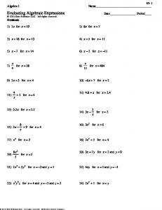
Worksheet by Kuta Software LLC. Algebra 1. ID: 1 ... E. Evaluating Algebraic
Expressions. Evaluate. 1) 2x for x = 19. 2) 8x for x = 7. 3) x + 18 for x = 13. 4) x + 5
...
receiving instruction in arithmetic and algebra, and one group in algebra without
.... instructor who taught both arithmetic and algebra in the Marathi language.
ALGEBRAIC EXPRESSIONS IN HANDW'OVEN TEXTILES Robert by Kirkpatrick
... Taking the cube of a binomial, I approached it in the way applied algebraic.
Algebraic expressions are made up of constants and variables connected by are
made ... Then, we can represent a verbal phrase as an algebraic expression.
symbols, tables, and area representations of algebraic expressions. It will help
you to identify and support students who have difficulty: • Recognizing the order
of ...
Optimized Translation of XPath into Algebraic Expressions ... - CiteSeerX
The goals of the approach are 1) to enable pipelined evaluation, 2) to avoid producing duplicate ... init program) produces the first result tuple. One can think of ...
Optimized Translation of XPath into Algebraic Expressions Parameterized by Programs Containing Navigational Primitives Sven Helmer [email protected]
Abstract We propose a new approach for the efficient evaluation of XPath expressions. This is important, since XPath is not only used as a simple, stand-alone query language, but is also an essential ingredient of XQuery and XSLT. The main idea of our approach is to translate XPath into algebraic expressions parameterized with programs. These programs are mainly built from navigational primitives like accessing the first child or the next sibling. The goals of the approach are 1) to enable pipelined evaluation, 2) to avoid producing duplicate (intermediate) result nodes, 3) to visit as few document nodes as possible, and 4) to avoid visiting nodes more than once. This improves the existing approaches, because our method is highly efficient.
1 Introduction XPath is an essential ingredient of mainstream XML applications like XSLT and XQuery. Moreover, XPath is often used as a simple query language itself. This motivated us to take a close look at efficient evaluation strategies for XPath and come up with a new approach. Standard XPath evaluators like Xalan or XT, for example, perform an evaluation that processes the location steps in an XPath expression from left to right, step by step. For n nodes this leads to n intermediate results, which are then unioned. During unioning duplicate elimination is performed, the result of which is fed into the next location step. Thereby, the result of every location step is materialized. Besides other advantages, our approach allows a pipelined evaluation of XPath expressions. Pipelining, which avoids building intermediate results, is one of the major reasons why query evaluation in relational database systems is highly efficient. Our goal was to realize pipelined evaluation of XPath expressions. As we will see, several obstacles need to be overcome. The biggest one is that the results of
a location step applied to two different nodes are often not disjoint. Performing a duplicate elimination operation after every location step, however, jeopardizes any attempt at pipelined processing. 1.1 Problem
Let us illustrate the problem by a simple example. As every location step results in a set of nodes, a simple UnnestMap operation is the appropriate algebraic operator for representing a location step [10]. We use subscripts to denote the location step the operation refers to. Let l be a location step including a node test and possible predicates. Then UnnestMap$1:l (·) produces for every input node a set of output nodes that are reachable by l. The result nodes are successively bound to a variable or attribute named $1. We assume that attributes of tuples handed from one algebraic operator to another may not only have a basic type (like integer or string), but may also be of type node. More formally we can define UnnestMap$i:l (e) := {x ◦ [$i : y]|x ∈ e, y ∈ x/l} where $i is an attribute name, e a general XPath expression, and ◦ denotes tuple concatenation. It is important to note that this operator does not eliminate duplicates: as usual in standard relational algebra implementations we assume a bag semantics for our algebraic operators. We now take a look at a straightforward translation of the XPath expression //A//A into a sequence of UnnestMap operations: UnnestMap$2:desc::A (UnnestMap$1:desc::A (·)). If this expression is applied to the document root node of an XML document that is a binary tree of elements of type A only, this expression clearly produces duplicates. Moreover, its runtime is quadratic in the number of nodes of the input document. In general, a straightforward translation of an XPath expression results in a sequence of UnnestMap operations, where plenty of duplicates can occur. Since the XPath specification demands set semantics, we need a final duplicate elimination in order to ensure correctness. Still, a lot of duplicate work may be performed by UnnestMap operations following an intermediate result that contains duplicates. Introducing a duplicate elimination operation after every UnnestMap operation avoids the unnecessary work but jeopardizes pipelining, since duplicate elimination is a pipeline breaker. 1.2 Context
The above description of UnnestMap is given on a logical level. In a real implementation, algebraic operators are typically implemented as iterators providing open, next, and close methods [12]. The context of this work is the native XML database system Natix [14]. In Natix, algebraic operators are parameterized by programs written in an assembler-like language which are then interpreted by the Natix Virtual Machine (NVM). XML-related primitives allow simple navigations like getFirstChild, getNextSibling and the like. This is similar to DOM, for example, which also provides navigational primitives. Our approach carries over to all systems that support primitive navigations between nodes. In Natix, an UnnestMap operator is parameterized by three programs. The first program (called init program) produces the first result tuple. One can think of this program as being called by the open method. The second program (called step program) produces the next tuple of the output. It is called by the next method. Another program (responsible for cleaning up), which is of no importance for understanding this paper, is called by the close method. 2
1.3 Contributions and Approach
Our contribution is a translation mechanism from XPath expressions to programs for a sequence of UnnestMap operations such that 1. pipelined evaluation becomes possible, 2. no duplicates are produced, 3. as few document nodes as possible are visited, 4. the number of visits per document node is minimized, and 5. the result nodes are returned in document or reverse document order. In fact, we not only enable pipelined evaluation of XPath expressions, but are also often able to reduce the size of an intermediate result to one node. Although, in principle we are able to treat all axes of XPath, we have to apply some restrictions on the XPath expressions we treat in this paper. The reasons are complexity and space limitations. Nevertheless, the subset of XPath we treat is much larger than the subset containing only child and descendent axes typically treated in literature [2]. We achieve these ambitious goals in three steps. First we eliminate those axes by XPath rewrite that will hamper a smooth translation process. Then we rewrite XPath expressions again by introducing artificial step functions to enable further rewrites allowing uncomplicated code generation. In a last step, we translate the rewritten, enhanced XPath expressions into efficient programs. 1.4 Restrictions
The first restriction is that we do not allow position() and last() function calls in our XPath expressions. We do not elaborate on the namespace axis either since it can be treated similar to the attribute axis. The other restrictions can be roughly described as follows. We do not treat the preceding-sibling and following-sibling axes. Although our approach carries over to XPath expressions embedded in predicates, we will not detail their treatment. Last, the prefix of an XPath expression that precedes a following or preceding axis must – in the basic approach – adhere to some restrictions concerning the order in which axes may occur (see Sec. 3 for details). Section 6 will indicate how these restrictions can be lifted. However, we currently do not have an alternative solution to handle the ancestor axis if it is not followed by a following or preceding axis. In this case, we must rely on its straightforward computation followed by duplicate elimination. Note that this fallback to a straightforward evaluation with interspersed duplicate eliminations still remains an option for any case we cannot handle more efficiently. 1.5 Related Work
We are not alone in searching for efficient evaluation techniques of XPath. Several authors have been concerned with rewriting XPath expressions using only the child and descendent axis. They minimize these tree pattern queries [3, 17]. Work along this line can be used to preprocess XPath expressions and it is beneficial to apply these minimizations prior to our translation process. Since backward axes are impossible to evaluate on streaming XML, approaches exist to rewrite XPath expressions such that only forward axes are used [5, 16]. Again, this work is orthogonal to ours. In fact, we will use some of their rewrite rules to preprocess XPath expressions in our first step. 3
A standard evaluation procedure for XPath expressions that contain only child and descendent axes is to translate them into an automaton. This approach is described in [2, 6], for example. The focus here is on selective information dissemination. A generalization to more axes is still missing. Some optimizing rewrites can be applied to XPath expressions when the DTD of the queried documents is known [15]. Again, this work is orthogonal to ours and can be beneficially applied prior to our translation process. Gottlob et al. propose an evaluation strategy for general XPath expressions in [11]. The underlying idea is the same as in our approach: avoid duplicate evaluation. Their approach is similar to our NVM DupElim approach which pushes duplicate eliminations down the evaluation tree. However, the highest performance gains and the enabling of pipelining is achieved by our rewrite phase. [11] lack such a rewrite phase. Another advantage of our approach is that we produce results in document or reverse document order. Other evaluation strategies for XPath expressions build on relational representations of XML in conjunction with numbering schemes. One specific approach is to translate XPath into SQL (the latest here is [18]). Others are concerned with providing efficient join algorithms to evaluate a single location step [1]. The functions first and last, which we will introduce later, resemble some algebraic operators found in [8]. However, they do not consider translation of path expressions into their algebra but require the user to use their algebra as a query language. Also, they do not allow nested objects in their GC-lists, which are used for evaluating the algebra. Context sets in XPath may contain nested objects (e.g. nodes that are descendants of others). An orthogonal area of research considers the acceleration of XPath evaluation by using indexes [9, 13]. 1.6 Organization
The remainder of the paper is organized as follows. In Section 2 we introduce some preliminaries and the first simple rewrite steps to prepare XPath expressions for our purposes. The goal of the preliminary rewrite is to eliminate the axes that are not relevant to our work since their computation does not pose any problems, or the axes that disturb further rewrites. Section 3 introduces the notion of step functions that generalize location steps. Using the introduced step functions, we rewrite XPath expressions until they have a convenient form for code generation. The main goal here is to break down step functions in such a way that they operate on single location steps. Section 4 describes how code generation proceeds for the different location path functions. Section 5 presents some performance measurements. Section 6 shows how the restrictions mentioned above can be relaxed such that we are able to translate many more XPath expressions into optimized plans. Section 7 concludes the paper.
2. Preliminaries and Preparatory Rewrites 2.1. Notation, Abbreviations, Assumptions
We use α and β to denote XPath expressions. Node tests are denoted by n or m. For predicates we use p and q. In order to keep the XPath expressions in the paper short, we use desc, anc, prs, fos, fol, pre, and par as abbreviations for descendant, ancestor, preceding-sibling, following-sibling, following, preceding, and parent. We abbreviate -or-self by 4
1,20
2,7
3,4
8,13
14,19
5, 6 9,10
11,12 15,16
17,18
Each node is assigned the pair dmin, dmax. Figure 1. Depth-first numbering of document nodes
-os. Whenever we are not interested in the specific node test or predicates, we just omit them from the path expression. For the introduction of step functions we need a node numbering according to a depth-first traversal. We will denote by dmin the number that is assigned to a document node at the time of its first visit during a depth-first traversal. By dmax we denote the number that is assigned to a node upon the second (and last) visit. For a simple example document these numbers are given in Fig. 1. The traversal primitives implemented in the runtime system are assumed to support preorder traversal and its reverse (by an iterator concept). A runtime system supporting postorder traversal will speed up certain evaluation steps. Otherwise we have to emulate postorder traversal with preorder traversal. 2.2. Preparatory Rewrites
Since XPath contains 13 axes, we would like to cut down the number of axes considered in this paper. We do so without loss of generality. There are two problems. The first problem is that some axes produce duplicate nodes, even if the input set does not contain duplicates. This problem originates from the definition of XPath. The second problem has its origins in our approach. For some axes it is not easy to find efficient rewrites. If an axis does not pose any of these two problems, we can safely omit it from further considerations. The axes we can safely omit are self, namespace, and attribute. The self axis can be evaluated by applying a simple selection operation. The namespace and attribute axes do not generate duplicates if their input does not contain duplicates. Allowing these two axes to appear not only at the end of an XPath expression is a controversial topic (see XPath 1.0 specification [7] vs. XPath 2.0 specification [4]). When allowing further location steps after attribute and namespace axes, we can rewrite the path expressions such that without loss of generality these axes occur only at the end of XPath expressions, within a predicate or can be eliminated altogether (i.e., the answer set is emtpy). For the attribute axis the following cases can be handled very easily, since their answer set is empty: attribute :: n[p]/desc :: m[q] = ∅ attribute :: n[p]/child :: m[q] = ∅ attribute :: n[p]/fol :: m[q] = ∅ 5
We can rewrite the remaining combinations of the attribute axis with the other axes in the following way: attribute :: n[p]/anc :: m[q] ≡ self :: ∗[attribute :: n[p]]/anc-os :: m[q] attribute :: n[p]/anc-os :: m[q] ≡ self :: ∗[attribute :: n[p]]/anc-os :: m[q] | attribute :: n[p]/self :: m[q] attribute :: n[p]/desc-os :: m[q] ≡ attribute :: n[p]/self :: m[q] attribute :: n[p]/par :: m[q] ≡ self :: m[q][attribute :: n[p]] We now turn to the namespace axis. Again, we have a lot of cases where the answer set is empty, namely the following combinations: namespace :: n[p]/desc :: m[q] namespace :: n[p]/child :: m[q] namespace :: n[p]/fol :: m[q] namespace :: n[p]/fos :: m[q] namespace :: n[p]/pre :: m[q] namespace :: n[p]/prs :: m[q] namespace :: n[p]/attribute :: m[q] namespace :: n[p]/namespace :: m[q]
= = = = = = = =
∅ ∅ ∅ ∅ ∅ ∅ ∅ ∅
We can rewrite the remaining combinations of the namespace axis with the other axes in the following way: namespace :: n[p]/anc :: m[q] ≡ namespace :: ∗[attribute :: n[p]]/anc-os :: m[q] namespace :: n[p]/anc-os :: m[q] ≡ self :: ∗[namespace :: n[p]]/anc-os :: m[q] | namespace :: n[p]/self :: m[q] namespace :: n[p]/desc-os :: m[q] = namespace :: n[p]/self :: m[q] namespace :: n[p]/par :: m[q] = self :: m[q][namespace :: n[p]] In the latter four cases of the attribute and namespace axes, adding an UnnestMap operator accessing attributes or namespaces to the plan is straightforward. 6
The next two axes that are somewhat troublesome are following-sibling and preceding-sibling. These axes can produce duplicates even if their input does not contain duplicates. Although we are able to treat them (see Sec. 6), their evaluation is slightly less efficient than that of other axes. Fortunately, [16] provides rewrites to eliminate following-sibling and preceding-sibling if they are preceded by a backward axis. We add the following rewrite rules to eliminate further top-level occurrences: desc :: n/fos :: m ≡ desc :: m[prs :: n] child :: n/fos :: m ≡ child :: m[prs :: n] Remaining occurrences are handled as indicated in Sec. 6. Another axis that produces duplicates even if the input set does not contain them is parent. Again, occurrences of the parent axis within path expressions are not always handled smoothly by our approach. Hence, we eliminate as many occurrences as possible by rewrites. We add to the parent elimination rules of [16]: anc :: n[p]/par :: m[q] anc-os :: n[p]/par :: m[q] desc-os :: n[p]/par :: m[q] α/prs :: n[p]/par :: m[q]
Olteanu et al. also describe rules to eliminate anc axes in [16]. We add the following to these rules: ≡ α[prs :: n[p]]/anc :: m[q]
α/prs :: n[p]/anc :: m[q]
These rules either eliminate occurrences from the top level or move them one step further to the front of the XPath expression where they are possibly eliminated. Occurrences at the very beginning of an XPath expression can be handled easily (as root nodes neither have parents nor ancestors). There are several optimizing rewrites possible for XPath expressions. We can apply them beneficially before proceeding with our optimized translation procedure. Minimization of occurring tree patterns is one of them [3, 17]. Another example is to replace desc-os :: ∗/child :: x[p] by desc :: x[p]. This is an important rewrite, since the first form (abbreviated as //x[p] in XPath) occurs quite frequently. Other techniques such as exploiting DTDs for rewrites (see [15]) should also be applied.
3. Step Function based Rewrite In terms of the number of nodes visited, the axes desc, desc-os, fol, and pre are the most expensive ones. Further, for all input sets with a cardinality larger than one all these axes produce duplicates with a high probability. Hence, we subsequently concentrate on these axes and try to make their evaluation as efficient as possible. Let us give a motivationg example. Suppose that we want to evaluate the expression α/fol :: n[p]. Furthermore, assume that the set of context nodes defined by α consists of two nodes (pictured in Figure 2). Evaluating the above expression separately for each node results in a lot of extra work (which increases even more for larger sets of context nodes). As the sets of following nodes overlap, it suffices to only look at the nodes following the context node with the smallest dmax value. 7
By definition of XPath, the following axis of a node n contains all nodes whose dmin value is larger than the dmax value of n. Hence, it suffices to compute the following nodes of the node whose dmax value is minimal. A similar argument holds for computing all the preceding nodes of a given set of nodes: it suffices to compute all preceding nodes of the node with the maximal dmin value. Let us formalize this idea. For a given set of nodes X and d ∈ {dmin, dmax} we define firstd (X) := {x|x ∈ X, x.d = min({y.d|y ∈ X})} lastd (X) := {x|x ∈ X, x.d = max({y.d|y ∈ X})} We call these functions step functions since we will treat them like “regular” steps within path expressions. The semantics of a step function occurring in an (extended) XPath expression is that for every context node the argument of the step function (typically a path expression) is evaluated to a set of nodes. The result of the location step is the result of applying the step function to the set of nodes derived by evaluating the argument. More formally, we define the semantics of step function f occurring in a path expression α/f (β) as follows. Let α evaluate to the set X. Then [
α/f (β) :=
f (x/β)
x∈X
where x/β is the set of nodes reachable by the path expression β with x as the current node. For an arbitrary path expression α, we can make the following two important observations: α/fol = firstdmax (α)/fol α/pre = lastdmin (α)/pre Note that if we can compute firstdmax efficiently, no duplicates will be generated by computing the subsequent following axis. Moreover, instead of computing all result nodes for α, it suffices to 8
compute only one! Both savings can dramatically reduce the evaluation costs of an XPath expression containing a following or preceding axis. Let us now turn to the descendant and descendant-os axis. Their treatment in our approach is identical. The question we have to answer first is in which situations descendant or descendant-os generate duplicates. This is the case whenever two nodes exist in the input set such that one is the ancestor of the other. If there are no such nodes, we can be sure that we do not produce duplicates. Exploiting this feature leads to the next step function called roots. For a given set of nodes X, it is defined as follows: roots(X) := {x|x ∈ X, 6 ∃y ∈ X y is an ancestor of x} 3.2. Rewrite
We have replaced XPath expressions with expressions containing our step functions, which avoids the generation of duplicates. We now rewrite these expressions such that code generation becomes feasible. For this the following properties of step functions are very useful. Let s be a singleton location step, i.e. a location step that produces for a single input node at most one output node. Then, the following holds: firstd (s/α) = s/firstd (α) lastd (s/α) = s/lastd (α) roots(s/α) = s/roots(α)
(1) (2) (3)
Note that s can also be a step function that returns a single node such as first dmax . Another possibility is that s consists of an axis that produces a single node. Typical candidates are parent and self. Yet another possibility is to use DTD knowledge to infer that an axis can only return a single node. The usefulness of these equations is that we are able to move some steps out of our step functions. The rules above are a first step, but we need more complex rules to fully rewrite path expressions. Therefore we introduce step functions where possibly large chunks of the original path expression become arguments. Since these are difficult to handle during code generation, more rules are needed to distribute step functions over complex path expressions such that their arguments become less complex path expressions. In case of first and last, we rewrite until their arguments are single steps. For roots we rewrite until the argument path starts with a descendant-os or descendant axis followed by an arbitrary number of occurrences of child. Let us define the set of down-axes as D := {desc, desc-os, self, child} and the set of specially processed axes as S := {fol, pre, desc, desc-os}. Consider a path expression of the form α/s/β where s is the last location step that is a member of S. Then we introduce our step functions by applying one of the following rewrite rules: α/fol/β α/pre/β α/desc/β α/desc-os/β
If β contains an axis not in D, special care is taken to eliminate duplicates as early as possible (e.g. for the anc or par axis). 9
After introducing a step function, its argument is the possibly complex path expression α. Subsequently, we have to simplify α such that code generation becomes possible. We first rewrite the argument of a roots(α) expression. In doing so, occurrences of first and last may be introduced. We apply the following rules: roots(α/fol/β) = firstdmax (α)/anc-os/fos/ roots(desc-os/β) where β ⊆ D roots(α/pre/β) = lastdmin (α)/anc-os/prs/ roots(desc-os/β) where β ⊆ D roots(α/desc/β) = roots(α)/roots(desc/β) if β contains only child axes β may be empty roots(child/α) = child/roots(α) if α ⊆ D roots(parent/α) = parent/roots(α)
(8)
(9) (10)
(11) (12)
Eqn. 10 is also valid if desc-os is used instead of desc. After rewrite, we require that only paths of the form desc/child∗ or desc-os/child∗ occur as arguments of roots. Note that this is not always the case, for example, if fos occurs in α and is not followed by fol or pre. We now turn to simplifying the argument path of firstdmax (α) and lastdmin (α). The goal is to distribute firstd and lastd occurrences over α such that each of their argument paths has a length of exactly one (location step). In doing so it does not suffice to consider first dmax and lastdmin . We also exploit firstdmin and lastdmax . The rewrite rules are firstdmax (α/pre) = firstdmax (α[pre])/firstdmax (pre)
(The proofs of these rules can be found in Appendix A.) Each application of one of the rules removes a single location step from the argument path. This is repeated until the path length becomes one. The rules given above do not cover all cases, but are the ones that can be easily described in terms of nondeterministic finite automata. (We will see in Section 6 how to treat the other cases.) The rules indicate which transitions are possible (see Figure 3). The states of the automata are firstdmax , firstdmin , lastdmin , and lastdmax . These are denoted by [f |l][dmax|dmin]. The start states are fdmax and ldmin. All states are final states. Consequently, the path that occurs as an argument of firstd or lastd can be acceptably rewritten if its reverse is accepted by the automata in Fig. 3. If the path expression is accepted by the automata, we have a simple way to rewrite the extended path expression such that a firstd or lastd is applied only to a single location step. This eases code generation since we only have to supply code fragments for every combination of these two functions, their possible subscripts dmin and dmax, and the XPath axes. Together with the code generation of roots(desc/child/ . . . /child), this is the subject of the next section. 3.3. Example rewrite
We rewrite the sample path /desc :: a/anc :: b/desc :: c/fol :: d/ desc :: e/child :: f /child :: g. First, we introduce the roots step function using Eqn. 6, since the last interesting axis is desc. This yields roots(/desc :: a/anc :: b/desc :: c/fol :: d)/ desc :: e/child :: f /child :: g The path in roots contains a fol axis. Hence, we introduce a firstdmax using Eqn 4: roots(firstdmax (/desc :: a/anc :: b/desc :: c)/ fol :: d)/desc :: e/child :: f /child :: g The next step is to move firstdmax out of roots using Eqn. 3: firstdmax (/desc :: a/anc :: b/desc :: c)/ roots(fol :: d)/desc :: e/child :: f /child :: g Next, we distribute first over the steps using Eqn. 19 which yields 11
firstdmin (/desc :: a/anc :: b[desc :: c])/ firstdmax (desc :: c). Then we apply Eqn. 18 firstdmin (/desc :: a[anc :: b[desc :: c]])/ firstdmin (anc :: b[desc :: c])/firstdmax (desc :: c) Call this expression α. We expand the fol axis: roots(anc :: ∗/fos :: ∗/desc-os :: d)/desc :: e/ child :: f /child :: g which is equivalent to: anc :: ∗/fos :: ∗/roots(desc-os :: d)/desc :: e/ child :: f /child :: g A sequence of interleaved first sequences recognized by the nested predicates (as in α) is translated into a single UnnestMap. Its programs avoid duplicate evaluation of those paths that are contained in the predicates as well as in the subsequent top-level path. The plan for our example path is shown in Fig. 4. Note, that this plan is fully pipelined, α can be evaluated very efficiently and returns only a single node, and no duplicates are produced in any step. The next section will show how to translate the subscripts of the plan into init and step programs. Note that the top three UnnestMap operations can be handled together to make the program more efficient.
4. Code Generation As we have seen in the last section, two important patterns emerged for which we want to be able to generate efficient code. One is an UnnestMap with a sequence of interleaved first d (or lastd ) sequences. The other is an UnnestMap for a root step operating on a descendant axis followed by several child 12
UnnestMap[$7 : $6/child :: g] | UnnestMap[$6 : $5/child :: f ] | UnnestMap[$5 : $4/desc :: e] | UnnestMap[$4 : $3/roots(desc-os :: d)] | UnnestMap[$3 : $2/fos :: ∗] | UnnestMap[$2 : $1/anc :: ∗] | UnnestMap[$1 : $0/α] | Some Input Document[root = $0] Figure 4. A Fully Pipelined Plan for the Sample Path
axes. We generate code for the operations open (called init in our case) and next (called step in our case) of an iterator allowing pipelined processing. The program for init initializes an iterator and hands back the first qualifying node. Each call of next returns the next qualifying node. We start with the code generation for a sequence of firstd (lastd steps are handled analogously). Then we consider the example programs for handling a firstdmin with a descendant axis. A complete list of programs can be found in Appendix C. Input to the code generation is the current context node cn[0] and a sequence of steps (with the individual steps stored in an array step[] and the corresponding predicates in an array pred[]). The steps of a sequence are processed from left to right, so we do not know yet for an intermediate node, if, after applying the remaining steps, any qualifying nodes exist. That means, that during evaluation of a sequence we may have to backtrack. For this reason we use two subroutines in our code generation algorithm: one to find the first node for a step, called mini-init and another one to find subsequent nodes, called mini-step. The subroutine mini-init(cn, step, pred) has as its output the first qualifying node for a given context node, a firstd step, and its predicates. The subroutine mini-step(cn orig, cn current, step, pred) navigates to the next qualifying node given the original context node from mini-init, a (qualifying) starting node, a first d step and its predicates (again excluding predicates concerning later steps). Let us now present the init part of the algorithm for the code generation of first d steps: init: cn[1] = mini-init(cn[0], step[1], pred[1]); label1: if(cn[1] == NULL) { return NULL; } 13
cn[2] = mini-init(cn[1], step[2], pred[2]); label2: if(cn[2] == NULL) { cn[1] = mini-step(cn[0], cn[1], step[1], pred[1]); goto label1; } ... cn[n] = mini-init(cn[n-1], step[n], pred[n]); labeln: if(cn[n] == NULL) { cn[n-1] = mini-step(cn[n-2], cn[n-1], step[n-1], pred[n-1]); goto labeln-1; } return cn[n]; The UnnestMap operator for a sequence of firstd steps returns at most one qualifying node. So the step program is very simple, it always returns NULL, as the lone potential node is already returned by the init program. In order to get a feel for the mini-init and mini-step programs, we present the programs for a firstdmin step with a descendant axis. For the mini-init program we just have to step through the descendants of the current context node in preorder. The first node qualifying the predicates is returned. mini-init(cn, first_dmin(desc), pred) { mini-init: start = cn; if(nextpreorder(start) does not exist) return NULL; next = nextpreorder(start); label: if(next is not descendant of start) return NULL; if(next satisfies pred) return next; if(nextpreorder(next) does not exist) return NULL; next = nextpreorder(next); goto label; } } The corresponding step program traverses the subsequent qualifying nodes in preorder.
14
mini-step(cn_orig, cn_current, first_dmin(desc), pred) { mini-step: start = cn_current; if(nextpreorder(start) does not exist) { return NULL; } next = nextpreorder(start); label: if(next is not descendant of cn_orig) { return NULL; } if(next satisfies pred) { return next; } if(nextpreorder(next) does not exist) { return NULL; } next = nextpreorder(next); goto label; } } Note that the two procedures for the init and step program are very similar. However, since our UnnestMap operator takes these programs as different parameters, we don’t generalize these programs to a single one.
5. Evaluation In this section we present a first round of experiments, which were performed to validate the effectiveness of our technique. The experimental environment was an Intel Pentium II with 400 MHz, running Linux 2.4. The tests used Natix’ query execution engine, the Natix Virtual Machine (NVM), written in C++ and compiled with optimizing gcc 3.1. As a reference, the same XPath expressions were also evaluated with the Xalan XSLT processor, also compiled with optimizing gcc, and using a very simple stylesheet which only selects the nodes reachable by the given XPath expression, doing nothing with them. We evaluated four different XPath expressions, using the same three XML documents each time, and starting from the document root node as context node. The documents were of a simple recursive structure with a fixed fanout on each inner node, with a constant tree height of five. All the nodes carried the same tag name, and the leaf nodes were empty tags with no text. The results are shown in Figure 5. The measurements of evaluation times were averaged over a series of program runs and do not include the overhead caused by program startup. These overhead times are shown at the bottom of the table. For Xalan, they grow with the document size because the document must be parsed first, while in Natix it is already stored as a tree structure. 15
The queries are shown in the table as a sequence of axes, using the abbreviations from Sec. 2. The node test used for each location step is always the same tag name (the one from the document). The first expression is only shown as a reference. It computes all descendants of the document root. No intermediate results are generated. Xalan is faster than a simple NVM UnnestMap because NVM operates directly on the secondary storage structure while Xalan navigates using main memory pointers, and the effort for parsing the document in Xalan is not included in the numbers. The second expression consists of two descendant axes. The three evaluation methods shown are NVM using a final duplicate elimination operator to eliminate duplicates (NVM DupElim), using a pipelined plan as explained in sections 3 and 4 (NVM Pipe), and using Xalan. The pipelined execution outperforms the other evaluation methods by factors up to 2.5. The third expression combines a descendant with a following axis, resulting in the generation of a large repeating node sequence from the following step in the conventional methods (NVM DupElim and Xalan), which is subject to duplicate elimination. The pipelined version (NVM Pipe) still exhibits performance figures close to a single tree traversal. In the last path expression, the third XPath expression was extended by another descendant axis. We used two approaches without pipelining here, differing in the point of time when the duplicates are eliminated. We can either use only a final duplicate elimination operator (NVM DupElim), or push another duplicate elimination into the execution plan after the first two axes have been evaluated (NVM Push). Pushing a second duplicate elimination is already an improvement, reducing the number of intermediate nodes considerably. This brings the execution time of the last expression down close to the execution time of the third expression with a single duplicate elimination. Xalan’s performance figures indicate that it does not perform an intermediate duplicate elimination (as also pointed out in [11]). The pipelined execution performance is still in the vicinity of a single tree traversal, making it several 16
thousand times faster than NVM DupElim, NVM Push and Xalan. Summarizing, the first experimental evaluation of pipelined XPath is very promising. It is our intention to verify the robustness of our technique against different selectivities of node tests, and against different classes of document structure.
6. Extensions Let us reexamine the restrictions mentioned in the introduction. Out of our equivalences, only Eqns. 4 to 7 pose any problems for occurrences of position() or last(). They do so, if the predicate of the axis in S that is used as the anchor point contains one of these functions. It is easy to verify that any other occurrence does not pose any problems. The other restrictions have to do with the rewriting step functions. The automata in Fig. 3 do not accept the full XPath language. We now show how additional transitions can be added to rectify this situation. As an example let us consider the par axis. Assume that we want to compute firstdmax (α/par). Unfortunately, this is neither equal to firstdmax (α[par])/firstdmax (par) nor equal to firstdmin (α[par])/firstdmax (par). However, we are able to show that firstdmax (α/par) ∈ firstdmax (α[par])/first dmax (par)/desc-os
So, either we computed the correct node by computing firstdmax (α[par])/firstdmax (par) or firstdmin (α[par])/firstdmax (par), or we have to start over and search for the correct solution underneath the computed node (i.e., among its descendants). We iterate this procedure until no further qualifying nodes can be found in the descendants of the current solution. It is relatively easy to adapt the code generation procedure to handle this case. Our goal is completing the automata to accept the full XPath language (i.e., all axes). We give rules for all remaining axes in Appendix B, although not all rules will be as simple as those for the par axis. The only axis that still poses problems is the ancestor axis. Currently, we do not have an elegant solution within our framework. Hence, we plan to implement a special algebraic operator that computes all ancestors for a given set of nodes and concurrently performs duplicate elimination.
7. Conclusion We presented an approach for the efficient evaluation of XPath expressions by pipelining the individual location steps. This is not straightforward, as several difficulties have to be overcome. Among these are duplicate elimination and cutting down massively on the number of nodes visited. We reach our goal via extensive transformations of the original XPath expression allowing uncomplicated code generation. In addition to theoretical work, we implemented a prototype of our approach in our native XML database system Natix. The conducted experiments demonstrate the dominance of our approach in terms of performance. We were always faster than other methods, typically up to several orders of magnitude. We are optimistic that the few points remaining open can be settled in a satisfying manner and that pipelining is the right approach for efficiently processing XPath expressions. 17
Acknowledgment We thank Simone Seeger for her help in preparing the manuscript and the anonymous referees for their helpful comments.
References [1] S. Al-Khalifa, H. Jagadish, N. Koudas, J. Patel, D. Srivastava, and Y. Wu. Structural joins: A primitive for efficient XML query pattern matching. In Proc. IEEE Conference on Data Engineering, pages 141–152, 2002. [2] M. Altinel and M. Franklin. Efficient filtering of XML documents for selective dissemination of information. In Proc. Int. Conf. on Very Large Data Bases (VLDB), pages 53–64, 2000. [3] S. Amer-Yahia, S. Cho, L. Lakshmanan, and D. Srivastava. Efficient algorithms for minimizing tree pattern queries. In Proc. of the ACM SIGMOD Conf. on Management of Data, pages 497–508, 2001. [4] A. Berglund, S. Boag, D. Chamberlin, M. Fernandez, M. Kay, J. Robie, and J. Sim´eon. XML path language (XPath) version 2.0. Technical report, World Wide Web Consortium (W3C) Working Draft, 2002. [5] F. Bry, D. Olteanu, H. Meuss, and T. Furche. Symmetry in XPath. Technical Report PMS-FB-2001-16, LMU, M¨unchen, 2001. [6] C. Chan, P. Felber, M. Garofalakis, and R. Rastogi. Efficient filtering of XML documents with XPath. In Proc. IEEE Conference on Data Engineering, pages 235–244, 2002. [7] J. Clark and S. DeRose. XML path language (XPath) version 1.0. Technical report, World Wide Web Consortium (W3C) Recommendation, 1999. [8] C. Clarke, G. Cormack, and F. Burkowski. An algebra for structured text search and a framework for its implementation. The Computer Journal, 38(1):43–56, 1995. [9] T. Fiebig and G. Moerkotte. Evaluating Queries on Structure with eXtended Access Support Relations. In D. Suciu and G. Vossen, editors, The World Wide Web and Databases, LNCS 1997, pages 125–136. Springer, 2001. [10] T. Fiebig and G. Moerkotte. Algebraic XML construction and its optimization in Natix. World Wide Web Journal, 4(3):167–187, 2002. [11] G. Gottlob, C. Koch, and R. Pichler. Efficient algorithms for processing XPath queries. In Proc. Int. Conf. on Very Large Data Bases (VLDB), pages 95–106, 2002. [12] G. Graefe. Query evaluation techniques for large databases. ACM Computing Surveys, 25(2), June 1993. [13] T. Grust. Accelerating XPath location steps. In Proc. of the ACM SIGMOD Conf. on Management of Data, pages 109–120, 2002. [14] C.-C. Kanne and G. Moerkotte. Efficient storage of XML data. In Proc. IEEE Conference on Data Engineering, page 198, 2000. [15] A. Kwong and M. Gertz. Schema-based optimization of XPath expressions. Technical report, UC Davis, 2002. [16] D. Olteanu, H. Meuss, T. Furche, and F. Bry. XPath: Looking forward. In Workshop on XML-Based Data Management (XMLDM) in conjunction with EDBT, 2002. [17] P. Ramanan. Efficient algorithms for minimizing tree pattern queries. In Proc. of the ACM SIGMOD Conf. on Management of Data, pages 299–309, 2002. [18] I. Tatarinov, S. Viglas, K. Beyer, J. Shanmugasundaram, E. Shekita, and C. Zhang. Storing and querying ordered XML using a relational database system. In Proc. of the ACM SIGMOD Conf. on Management of Data, pages 204–215, 2002.
18
A Proofs of Step Rewrite Rules In this section we present the proofs for the rewrite rules from Section 3.2. Proof of Equation (13) Let x = firstdmax (α/pre). Then surely, x = firstdmax (α[pre]/pre). Also, if we only look at the predecessors with the minimal dmax value of each node, this will not hurt us either: x = firstdmax (α[pre]/firstdmax (pre)). y = firstdmax (α[pre])/firstdmax (pre) We now have to prove x = y: Let us assume that x 6= y. Let X = α[pre]/firstdmax (pre). As firstdmax (α[pre]) ∈ α[pre], obviously y ∈ X. We also know that x = firstdmax (X). As x 6= y and x has smallest dmax in X, we have x.dmax < y.dmax (i) With zy = firstdmax (α[pre]), y = zy /firstdmax (pre). y is a predecessor of zy , so y.dmax < zy .dmin (ii) Because of (i) and (ii), we also know x.dmax < zy .dmin, so x ∈ zy /pre. Since y is the predecessor of zy with the smallest dmax value, we have x.dmax > y.dmax. This contradicts (i). So x = y. Proof of Equation (14) x = firstdmax (α[pre]/firstdmax (pre)). y = firstdmin (α[pre])/firstdmax (pre) We now have to prove x = y: Let us assume that x 6= y. Let X = α[pre]/firstdmax (pre). Again, y ∈ X and x = firstdmax (X). As x 6= y, we have x.dmax < y.dmax (i) With zy = firstdmin (α[pre]), y = zy /firstdmax (pre). y is a predecessor of zy , so y.dmax < zy .dmin (ii) Because of (i) and (ii), we also know x.dmax < zy .dmin, so x ∈ zy /pre. Since y is the predecessor of zy with the smallest dmax value, we have x.dmax > y.dmax. This contradicts (i). So x = y. Proof of Equation (15) x = firstdmax (α[fol]/firstdmax (fol)). y = firstdmax (α[fol])/firstdmax (fol) We now have to prove x = y: Let us assume that x 6= y. Let X = α[fol]/firstdmax (fol). So, y ∈ X and x = firstdmax (X). As x 6= y, we have x.dmax < y.dmax (i) 19
Let zx be any node in α[fol], such that x = zx /firstdmax (fol). Let zy = firstdmax (α[fol]), i.e., y = zy /firstdmax (fol). Because zy has smallest dmax in α[fol], we know zy .dmax ≤ zx .dmax ∀zx (ii) As x ∈ zx /fol, zx .dmax < x.dmin (iii) From (ii) and (iii) we can deduce zy .dmax < x.dmin, so x ∈ zy /fol. However, y has smallest dmax in zy /(fol), so y.dmax < x.dmax. This contradicts (i). So x = y. Proof of Equation (16) x = firstdmin (α[fol]/firstdmin (fol)) y = firstdmax (α[fol])/firstdmin (fol) We now have to prove x = y: Let us assume that x 6= y. Let X = α[fol]/firstdmin (fol). So, y ∈ X and x = firstdmin (X). As x 6= y, we have x.dmin < y.dmin (i) Let zx be any node in α[fol], such that x = zx /firstdmin (fol). Let zy = firstdmax (α[fol]), i.e., y = zy /firstdmin (fol). Because zy has smallest dmax in α[fol], we know zy .dmax ≤ zx .dmax ∀zx (ii) As x ∈ zx /fol, zx .dmax < x.dmin (iii) From (ii) and (iii) we can deduce zy .dmax < x.dmin, so x ∈ zy /fol. However, y has smallest dmin in zy /(fol), so y.dmin < x.dmin. This contradicts (i). So x = y. Proof of Equation (17) x = firstdmin (α[anc]/firstdmin (anc)) y = firstdmax (α[anc])/firstdmin (anc) We now have to prove x = y: Let us assume that x 6= y. Let X = α[anc]/firstdmin (anc). So, y ∈ X and x = firstdmin (X). As x 6= y, we have x.dmin < y.dmin (i) Let zx be any node in α[anc], such that x = zx /firstdmin (anc). Let zy = firstdmax (α[anc]), i.e., y = zy /firstdmin (anc). Because zy has smallest dmax in α[anc], we know zy .dmax ≤ zx .dmax ∀zx (ii) Because x ∈ zx /anc and y ∈ zy /anc, we have x.dmin < zx .dmin < zx .dmax < x.dmax and y.dmin < zy .dmin < zy .dmax < y.dmax (iii) Putting (i), (ii), and (iii) together we get:
20
x.dmax. This contradicts (i). So x = y. Proof of Equation (26) x = lastdmin (α[pre]/lastdmin (pre)). y = lastdmin (α[pre])/lastdmin (pre) We now have to prove x = y: Let us assume that x 6= y. Let X = α[pre]/lastdmin (pre). So, y ∈ X and x = lastdmin (X). As x 6= y, we have x.dmin > y.dmin (i) Let zx be any node in α[pre], such that x = zx /lastdmin (pre). Let zy = lastdmin (α[pre]), i.e., y = zy /lastdmin (pre). Because zy has largest dmin in α[pre], we know zy .dmin ≥ zx .dmin ∀zx (ii) As x ∈ zx /pre, zx .dmin > x.dmax (iii) From (ii) and (iii) we can deduce zy .dmin > x.dmax, so x ∈ zy /pre. However, y has largest dmin in zy /(pre), so y.dmin > x.dmin. This contradicts (i). So x = y. Proof of Equation (27) x = lastdmin (α[fol]/lastdmin (fol)). y = lastdmax (α[fol])/lastdmin (fol) We now have to prove x = y: Let us assume that x 6= y. Let X = α[fol]/lastdmin (fol). So, y ∈ X and x = lastdmin (X). As x 6= y, we have x.dmin > y.dmin (i) With zy = lastdmax (α[fol]), y = zy /lastdmin (fol). y is a follower of zy , so y.dmin > zy .dmax (ii) Because of (i) and (ii), we also know x.dmin > zy .dmax, so x ∈ zy /f ol. Since y is the follower of zy with the largest dmin value, we have y.dmin > x.dmin. This contradicts (i). So x = y. Proof of Equation (28) x = lastdmin (α[fol]/lastdmin (fol)). y = lastdmin (α[fol])/lastdmin (fol) We now have to prove x = y: Let us assume that x 6= y. 25
Let X = α[fol]/lastdmin (fol). So, y ∈ X and x = lastdmin (X). As x 6= y, we have x.dmin > y.dmin (i) With zy = lastdmin (α[fol]), y = zy /lastdmin (fol). y is a follower of zy , so y.dmin > zy .dmax (ii) Because of (i) and (ii), we also know x.dmin > zy .dmax, so x ∈ zy /f ol. Since y is the follower of zy with the largest dmin value, we have y.dmin > x.dmin. This contradicts (i). So x = y. Proof of Equation (29) x = lastdmax (α[anc]/lastdmax (anc)) y = lastdmax (α[anc])/lastdmax (anc) We now have to prove x = y:
y.dmax (i) Let zx be any node in α[anc], such that x = zx /lastdmax (anc). Let zy = lastdmax (α[anc]), i.e., y = zy /lastdmax (anc). Because zy has largest dmax in α[anc], we know zy .dmax ≥ zx .dmax ∀zx (ii) Because x ∈ zx /anc and y ∈ zy /anc, we have x.dmin < zx .dmin < zx .dmax < x.dmax and y.dmin < zy .dmin < zy .dmax < y.dmax (iii) Putting (i), (ii), and (iii) together we get: x.dmin < zx .dmin < zx .dmax < x.dmax y.dmin < zy .dmin < zy .dmax < y.dmax It follows that x ∈ zy /anc, since x.dmin < zy .dmax < x.dmax However, y has largest dmax in zy /(anc), so y.dmax > x.dmax. This contradicts (i). So x = y. Proof of Equation (30) x = lastdmax (α[anc]/lastdmax (anc)) y = lastdmin (α[anc])/lastdmax (anc) We now have to prove x = y: Let us assume that x 6= y. Let X = α[anc]/lastdmax (anc). So, y ∈ X and x = lastdmax (X). As x 6= y, we have x.dmax > y.dmax (i) Let zx be any node in α[anc], such that x = zx /lastdmax (anc). Let zy = lastdmin (α[anc]), i.e., y = zy /lastdmax (anc). Because zy has largest dmin in α[anc], we know
26
x.dmax. This contradicts (i). So x = y. Proof of Equation (31) x = lastdmax (α[desc]/lastdmax (desc)) y = lastdmax (α[desc])/lastdmax (desc) We now have to prove x = y:
≥
y.dmax (i) Let zx be any node in α[desc], such that x = zx /lastdmax (desc). Let zy = lastdmax (α[desc]), i.e., y = zy /lastdmax (desc). Because zy has largest dmax in α[desc], we know zy .dmax ≥ zx .dmax ∀zx (ii) Because x ∈ zx /desc and y ∈ zy /desc, we have zx .dmin < x.dmin < x.dmax < zx .dmax and zy .dmin < y.dmin < y.dmax < zy .dmax (iii) Putting (i), (ii), and (iii) together we get: zx .dmin < x.dmin < x.dmax < zx .dmax zy .dmin < y.dmin < y.dmax < zy .dmax It follows that x ∈ zy /desc, since zy .dmin < x.dmax < zy .dmax However, y has the largest dmax in zy /(desc), so y.dmax > x.dmax. This contradicts (i). So x = y. Proof of Equation (32) x = lastdmin (α[desc]/lastdmin (desc)) y = lastdmax (α[desc])/lastdmin (desc) We now have to prove x = y: Let us assume that x 6= y. Let X = α[desc]/lastdmin (desc). So, y ∈ X and x = lastdmin (X). As x 6= y, we have x.dmin > y.dmin (i) Let zx be any node in α[desc], such that x = zx /lastdmin (desc). Let zy = lastdmax (α[desc]), i.e., y = zy /lastdmin (desc). 27
x.dmin. This contradicts (i). So x = y. Proof of Equation (33) x = lastdmax (α[anc-os]/lastdmax (anc-os)) y = lastdmax (α[anc-os])/lastdmax (anc-os) We now have to prove x = y:
y.dmax (i) Let zx be any node in α[anc-os], such that x = zx /lastdmax (anc-os). Let zy = lastdmax (α[anc-os]), i.e., y = zy /lastdmax (anc-os). Because zy has largest dmax in α[anc-os], we know zy .dmax ≥ zx .dmax ∀zx (ii) Because x ∈ zx /anc-os and y ∈ zy /anc-os, we have x.dmin ≤ zx .dmin < zx .dmax ≤ x.dmax and y.dmin ≤ zy .dmin < zy .dmax ≤ y.dmax (iii) Putting (i), (ii), and (iii) together we get: x.dmin ≤ zx .dmin < zx .dmax ≤ x.dmax y.dmin ≤ zy .dmin < zy .dmax ≤ y.dmax It follows that x ∈ zy /anc-os, since x.dmin < zy .dmax ≤ x.dmax However, y has largest dmax in zy /(anc-os), so y.dmax > x.dmax. This contradicts (i). So x = y. Proof of Equation (34) x = lastdmax (α[anc-os]/lastdmax (anc-os)) y = lastdmin (α[anc-os])/lastdmax (anc-os) We now have to prove x = y: Let us assume that x 6= y. Let X = α[anc-os]/lastdmax (anc-os). So, y ∈ X and x = lastdmax (X). As x 6= y, we have x.dmax > y.dmax (i) Let zx be any node in α[anc-os], such that x = zx /lastdmax (anc-os). 28
x.dmax. This contradicts (i). So x = y. Proof of Equation (35) x = lastdmax (α[desc-os]/lastdmax (desc-os)) y = lastdmax (α[desc-os])/lastdmax (desc-os) We now have to prove x = y:
≥
y.dmax (i) Let zx be any node in α[desc-os], such that x = zx /lastdmax (desc-os). Let zy = lastdmax (α[desc-os]), i.e., y = zy /lastdmax (desc-os). Because zy has largest dmax in α[desc-os], we know zy .dmax ≥ zx .dmax ∀zx (ii) Because x ∈ zx /desc-os and y ∈ zy /desc-os, we have zx .dmin ≤ x.dmin < x.dmax ≤ zx .dmax and zy .dmin ≤ y.dmin < y.dmax ≤ zy .dmax (iii) Putting (i), (ii), and (iii) together we get: zx .dmin ≤ x.dmin < x.dmax ≤ zx .dmax zy .dmin ≤ y.dmin < y.dmax ≤ zy .dmax It follows that x ∈ zy /desc-os, since zy .dmin < x.dmax ≤ zy .dmax However, y has the largest dmax in zy /(desc-os), so y.dmax > x.dmax. This contradicts (i). So x = y. Proof of Equation (36) x = lastdmin (α[desc-os]/lastdmin (desc-os)) y = lastdmax (α[desc-os])/lastdmin (desc-os) We now have to prove x = y: Let us assume that x 6= y. Let X = α[desc-os]/lastdmin (desc-os). So, y ∈ X and x = lastdmin (X). As x 6= y, we have x.dmin > y.dmin (i) 29
x.dmin. This contradicts (i). So x = y. Proof of Equation (37) x = firstdmin (α[pre]/firstdmin (pre)). y = lastdmin (α[pre])/firstdmin (pre) We now have to prove x = y:
≥
>
Let us assume that x 6= y. Let X = α[pre]/firstdmin (pre). So, y ∈ X and x = firstdmin (X). As x 6= y, we have x.dmin < y.dmin (i) Let zx be any node in α[pre], such that x = zx /firstdmin (pre). Let zy = lastdmin (α[pre]), i.e., y = zy /firstdmin (pre). Because zy has largest dmin in α[pre], we know zy .dmin ≥ zx .dmin ∀zx (ii) Because x ∈ zx /pre and y ∈ zy /pre, we have x.dmin < x.dmax < zx .dmin < zx .dmax and y.dmin < y.dmax < zy .dmin < zy .dmax (iii) Putting (i), (ii), and (iii) together we get: x.dmin < x.dmax < zx .dmin < zx .dmax y.dmin < y.dmax < zy .dmin < zy .dmax It follows that x ∈ zy /pre, since x.dmax < zy .dmin. Since y is the predecessor of zy with the smallest dmin value, we have x.dmin > y.dmin. This contradicts (i). So x = y. Proof of Equation (38) x = firstdmin (α[pre]/firstdmin (pre)). y = lastdmax (α[pre])/firstdmin (pre) We now have to prove x = y: Let us assume that x 6= y. Let X = α[pre]/firstdmin (pre). So, y ∈ X and x = firstdmin (X). 30
≥
>
As x 6= y, we have x.dmin < y.dmin (i) Let zx be any node in α[pre], such that x = zx /firstdmin (pre). Let zy = lastdmax (α[pre]), i.e., y = zy /firstdmin (pre). Because zy has largest dmax in α[pre], we know zy .dmax ≥ zx .dmax ∀zx (ii) Because x ∈ zx /pre and y ∈ zy /pre, we have x.dmin < x.dmax < zx .dmin < zx .dmax and y.dmin < y.dmax < zy .dmin < zy .dmax (iii) Putting (i), (ii), and (iii) together we get: x.dmin < x.dmax < zx .dmin < zx .dmax y.dmin < y.dmax < zy .dmin < zy .dmax It follows that x.dmin < zy .dmin and x.dmax < zy .dmax. Additionally, x.dmax < zy .dmin, because x.dmax > zy .dmin results in a malformed XML document. Therefore, x ∈ zy /pre. Since y is the predecessor of zy with the smallest dmin value, we have x.dmin > y.dmin. This contradicts (i). So x = y. Proof of Equation (39) x = lastdmax (α[fol]/lastdmax (fol)). y = firstdmin (α[fol])/lastdmax (fol) We now have to prove x = y:
y.dmax (i) Let zx be any node in α[fol], such that x = zx /lastdmax (fol). Let zy = firstdmin (α[fol]), i.e., y = zy /lastdmax (fol). Because zy has smallest dmin in α[fol], we know zy .dmin ≤ zx .dmin ∀zx (ii) Because x ∈ zx /fol and y ∈ zy /fol, we have zx .dmin < zx .dmax < x.dmin < x.dmax and zy .dmin < zy .dmax < y.dmin < y.dmax (iii) Putting (i), (ii), and (iii) together we get: zx .dmin < zx .dmax < x.dmin < x.dmax zy .dmin < zy .dmax < y.dmin < y.dmax It follows that x.dmax > zy .dmax and x.dmin > zy .dmin. Additionally, x.dmin > zy .dmax, because x.dmin < zy .dmax results in a malformed XML document. Therefore, x ∈ zy /fol. However, y has the largest dmax in zy /fol, so y.dmax > x.dmax. This contradicts (i). So x = y. Proof of Equation (40) x = lastdmax (α[fol]/lastdmax (fol)). 31
y = firstdmax (α[fol])/lastdmax (fol) We now have to prove x = y:
y.dmax (i) Let zx be any node in α[fol], such that x = zx /lastdmax (fol). Let zy = firstdmax (α[fol]), i.e., y = zy /lastdmax (fol). Because zy has smallest dmax in α[fol], we know zy .dmax ≤ zx .dmax ∀zx (ii) Because x ∈ zx /fol and y ∈ zy /fol, we have zx .dmin < zx .dmax < x.dmin < x.dmax and zy .dmin < zy .dmax < y.dmin < y.dmax (iii) Putting (i), (ii), and (iii) together we get: zx .dmin < zx .dmax < x.dmin < x.dmax zy .dmin < zy .dmax < y.dmin < y.dmax It follows that x ∈ zy /fol, since x.dmin > zy .dmax. However, y has the largest dmax in zy /fol, so y.dmax > x.dmax. This contradicts (i). So x = y.
B Proofs of Extensions In this section we present the proofs for the extensions from Section 6. We start with the par axis and then treat the remaining axes. B.1 Parent Axis
B.1.1 firstdmax Proof of Equation (41) x = firstdmax (α[par]/firstdmax (par)) y = firstdmax (α[par])/firstdmax (par) We now have to prove x = y or x ∈ y/desc: Let us assume that x 6= y and x 6∈ y/desc. Let X = α[par]/firstdmax (par). So, y ∈ X and x = firstdmax (X). As x 6= y, we have x.dmax < y.dmax (i) Let zx be any node in α[par], such that x = zx /firstdmax (par). Let zy = firstdmax (α[par]), i.e., y = zy /firstdmax (par). Because zy has smallest dmax in α[par], we know zy .dmax ≤ zx .dmax ∀zx (ii) Because x ∈ zx /par and y ∈ zy /par, we have x.dmin < zx .dmin < zx .dmax < x.dmax and y.dmin < zy .dmin < zy .dmax < y.dmax (iii) Putting (i), (ii), and (iii) together we get: 32
zx .dmin
≤
Proof: Let us assume that x 6= y and ¬(y.dmin < zy .dmin < zy .dmax < x.dmin < zx .dmin < zx .dmax < x.dmax < y.dmax). From the proof of Equation (41) we know that x.dmin < zx .dmin < zx .dmax < x.dmax y.dmin < zy .dmin < zy .dmax < y.dmax We also know that zx 6= zy , as zx = zy implies x = y (which is a contradiction). Additionally, x 6= zy (because zy .dmax < x.dmax) and y 6= zx (because zx .dmax < y.dmax). But this is still a partial ordering, we want to have a look at all possible complete orderings. There are (at most) 7 different positions where we can insert zx .dmin and x.dmin, respectively. zx .dmin 6↓ ↓(1) 6↓ ↓(2) 6↓ 6↓ 6↓ y.dmin < zy .dmin < zy .dmax < zx .dmax < x.dmax < y.dmax 6↑ ↑(a) 6↑ ↑(b) 6↑ 6↑ 6↑ x.dmin The positions marked with 6↓ and 6↑ are impossible, as they will result in a malformed XML document. Let us now look at the remaining cases in turn: 1.
(a) y.dmin < x.dmin < zx .dmin < zy .dmin < zy .dmax < zx .dmax < x.dmax < y.dmax (x.dmin has to be smaller than zx .dmin, else we would have a malformed XML document.) This case leads to a contradiction, as it implies y ∈ zy /anc/anc/anc, but we know that y ∈ zy /par. (b) y.dmin < zx .dmin < zy .dmin < zy .dmax < x.dmin < zx .dmax < x.dmax < y.dmax Contradiction, zx .dmin cannot be smaller than x.dmin.
2.
(a) y.dmin < x.dmin < zy .dmin < zy .dmax < zx .dmin < zx .dmax < x.dmax < y.dmax This case leads to a contradiction, as it implies y ∈ zy /anc/anc, but we know that y ∈ zy /par. (b) y.dmin < zy .dmin < zy .dmax < x.dmin < zx .dmin < zx .dmax < x.dmax < y.dmax (x.dmin has to be smaller than zx .dmin, else we would have a malformed XML document.) This is a contradiction to our assumption.
Therefore, x = y or y.dmin < zy .dmin < zy .dmax < x.dmin < zx .dmin < zx .dmax < x.dmax < y.dmax.
34
Supplements to Equation (42) x = firstdmax (α[par]/firstdmax (par)) y = firstdmin (α[par])/firstdmax (par) We now prove that either x = y or y.dmin < zy .dmin < x.dmin < zx .dmin < zx .dmax < x.dmax < zy .dmax < y.dmax or y.dmin < (zy .dmin =)x.dmin < zx .dmin < zx .dmax < x.dmax(= zy .dmax) < y.dmax or y.dmin < zy .dmin < zy .dmax < x.dmin < zx .dmin < zx .dmax < x.dmax < y.dmax. Graphically, this means that we have the following relationships besides x = y: y child
zy
y desc
y
x
zy
x=zy
child
zx
child
child
desc
x child
child
zx
zx
Proof: Let us assume that x 6= y and ¬(y.dmin < zy .dmin < x.dmin < zx .dmin < zx .dmax < x.dmax < zy .dmax < y.dmax) and ¬(y.dmin < x.dmin < zx .dmin < zx .dmax < x.dmax < y.dmax) and ¬(y.dmin < zy .dmin < zy .dmax < x.dmin < zx .dmin < zx .dmax < x.dmax < y.dmax).
>
≤
From the proof of Equation (42) we know that x.dmin < zx .dmin < zx .dmax < x.dmax y.dmin < zy .dmin < zy .dmax < y.dmax We also know that zx 6= zy , as zx = zy implies x = y (which is a contradiction). Additionally, y 6= zx (because zx .dmax < y.dmax). But this is still a partial ordering, we want to have a look at all possible complete orderings. There are (at most) 7 different positions where we can insert x.dmin and zy .dmax, respectively. x.dmin 6↓ ↓(1) ↓(2) 6↓ 6↓ 6↓ 6↓ y.dmin < zy .dmin < zx .dmin < zx .dmax < x.dmax < y.dmax 6↑ 6↑ ↑(a) 6↑ ↑(b) ↑(c) 6↑ zy .dmax The positions marked with 6↓ and 6↑ are impossible, as they will result in a malformed XML document. Let us now look at the remaining cases in turn: 1.
(a) y.dmin < x.dmin < zy .dmin < zy .dmax < zx .dmin < zx .dmax < x.dmax < y.dmax This case leads to a contradiction, as it implies y ∈ zy /anc/anc, but we know that y ∈ zy /par. (b) Here we have either y.dmin < x.dmin < zy .dmin < zx .dmin < zx .dmax < zy .dmax < x.dmax < y.dmax 35
or y.dmin < x.dmin = zy .dmin < zx .dmin < zx .dmax < zy .dmax = x.dmax < y.dmax The former is a contradiction, as it implies y ∈ zy /anc/anc, but we know that y ∈ zy /par. The latter contradicts our assumptions. (c) y.dmin < x.dmin < zy .dmin < zx .dmin < zx .dmax < x.dmax < zy .dmax < y.dmax Contradiction (malformed XML document, as x.dmin < zy .dmin and x.dmax < zy .dmax). 2.
(a) y.dmin < zy .dmin < zy .dmax < x.dmin < zx .dmin < zx .dmax < x.dmax < y.dmax (zy .dmax has to be smaller than x.dmin, else we would have a malformed XML document.) This contradicts our assumptions. (b) y.dmin < zy .dmin < x.dmin < zx .dmin < zx .dmax < zy .dmax < x.dmax < y.dmax Contradiction (malformed XML document, as zy .dmin < x.dmin and zy .dmax < x.dmax). (c) y.dmin < zy .dmin < x.dmin < zx .dmin < zx .dmax < x.dmax < zy .dmax < y.dmax This contradicts our assumptions.
B.1.2 Mapping firstdmin to firstdmax x = firstdmin (α[par]/firstdmin (par)) y = firstdmax (α[par])/firstdmin (par) We now prove that either x = y or x.dmin < zx .dmin < y.dmin < zy .dmin < zy .dmax < y.dmax < zx .dmax < x.dmax or x.dmin < (zx .dmin =)y.dmin < zy .dmin < zy .dmax < y.dmax(= zx .dmax) < x.dmax or x.dmin < y.dmin < zy .dmin < zy .dmax < y.dmax < zx .dmin < zx .dmax < x.dmax. Graphically, this means that we have the following relationships besides x = y: x child
zx
x desc
x
y
child
y
y=zx
child
child
zy
desc
child
zx
child
zy
zy
Proof: Let us assume that x 6= y and ¬(x.dmin < zx .dmin < y.dmin < zy .dmin < zy .dmax < y.dmax < zx .dmax < x.dmax) and ¬(x.dmin < y.dmin < zy .dmin < zy .dmax < y.dmax < x.dmax) and ¬(x.dmin < y.dmin < zy .dmin < zy .dmax < y.dmax < zx .dmin < zx .dmax < x.dmax). 36
As x 6= y, we have x.dmin < y.dmin (i) Because zy has smallest dmax in α[par] (and zy 6= zx ), we know zy .dmax < zx .dmax ∀zx (ii) Because x ∈ zx /par and y ∈ zy /par, we have x.dmin < zx .dmin < zx .dmax < x.dmax and y.dmin < zy .dmin < zy .dmax < y.dmax (iii) Putting (i), (ii), and (iii) together we get: x.dmin < zx .dmin < zx .dmax < x.dmax y.dmin < zy .dmin < zy .dmax < y.dmax Additionally, x 6= zy (because zy .dmax < x.dmax). Again we have a look at all possible complete orderings. There are (at most) 7 different positions where we can insert zx .dmin and y.dmax, respectively. zx .dmin 6↓ ↓(1) ↓(2) 6↓ ↓(3) 6↓ 6↓ x.dmin < y.dmin < zy .dmin < zy .dmax < zx .dmax < x.dmax 6↑ 6↑ 6↑ 6↑ ↑(a) ↑(b) 6↑ y.dmax The positions marked with 6↓ and 6↑ are impossible, as they will result in a malformed XML document. Let us now look at the remaining cases in turn: 1.
(a) We have either x.dmin < zx .dmin < y.dmin < zy .dmin < zy .dmax < y.dmax < zx .dmax < x.dmax or x.dmin < zx .dmin = y.dmin < zy .dmin < zy .dmax < y.dmax = zx .dmax < x.dmax. Both cases contradict our assumptions. (b) Either we have x.dmin < zx .dmin < y.dmin < zy .dmin < zy .dmax < zx .dmax < y.dmax < x.dmax or x.dmin < zx .dmin = y.dmin < zy .dmin < zy .dmax < zx .dmax = y.dmax < x.dmax. The former is a contradiction (malformed XML document, as zy .dmin < x.dmin and zy .dmax < x.dmax). The latter contradicts our assumptions.
2.
(a) x.dmin < y.dmin < zx .dmin < zy .dmin < y.dmax < zy .dmax < zx .dmax < x.dmax Contradiction (malformed XML document, as y.dmin < zx .dmin and y.dmax < zx .dmax). (b) We have either x.dmin < y.dmin < zx .dmin < zy .dmin < zy .dmax < zx .dmax < y.dmax < x.dmax or x.dmin < y.dmin = zx .dmin < zy .dmin < zy .dmax < zx .dmax = y.dmax < x.dmax. In the first case, we have a contradiction, as it implies y ∈ zy /anc/anc, but we know that y ∈ zy /par. The latter contradicts our assumptions.
(y.dmax has to be smaller than zx .dmin, else we would have a malformed XML document.) Contradiction to our assumptions. (b) x.dmin < y.dmin < zy .dmin < zy .dmax < zx .dmin < zx .dmax < y.dmax < x.dmax Contradiction, as it implies x ∈ zx /anc/anc, but we know that x ∈ zx /par. Therefore, x = y or x.dmin < zx .dmin < y.dmin < zy .dmin < zy .dmax < y.dmax < zx .dmax < x.dmax or x.dmin < (zx .dmin =)y.dmin < zy .dmin < zy .dmax < y.dmax(= zx .dmax) < x.dmax or x.dmin < y.dmin < zy .dmin < zy .dmax < y.dmax < zx .dmin < zx .dmax < x.dmax. B.1.3 Mapping firstdmin to firstdmin x = firstdmin (α[par]/firstdmin (par)) y = firstdmin (α[par])/firstdmin (par) We now prove that either x = y or x.dmin < y.dmin < zy .dmin < zy .dmax < y.dmax < zx .dmin < zx .dmax < x.dmax. Graphically, this means that we have the following relationship besides x = y: x desc
child
y
zx
child
zy
Proof: Let us assume that x 6= y and ¬(x.dmin < y.dmin < zy .dmin < zy .dmax < y.dmax < zx .dmin < zx .dmax < x.dmax). As x 6= y, we have x.dmin < y.dmin (i) Because zy has smallest dmin in α[par] (and zy 6= zx ), we know zy .dmin < zx .dmin ∀zx (ii) Because x ∈ zx /par and y ∈ zy /par, we have x.dmin < zx .dmin < zx .dmax < x.dmax and y.dmin < zy .dmin < zy .dmax < y.dmax (iii) Putting (i), (ii), and (iii) together we get: x.dmin < zx .dmin < zx .dmax < x.dmax y.dmin < zy .dmin < zy .dmax < y.dmax Additionally, x 6= zy (because x.dmin < zy .dmax) and y 6= zx (because y.dmin < zx .dmin. Again we have a look at all possible complete orderings. There are (at most) 7 different positions where we can insert zy .dmax and y.dmax, respectively. y.dmax 6↓ 6↓ 6↓ ↓(1) 6↓ ↓(2) 6↓ x.dmin < y.dmin < zy .dmin < zx .dmin < zx .dmax < x.dmax 6↑ 6↑ 6↑ ↑(a) 6↑ ↑(b) 6↑ zy .dmax 38
The positions marked with 6↓ and 6↑ are impossible, as they will result in a malformed XML document. Let us now look at the remaining cases in turn: 1.
(a) x.dmin < y.dmin < zy .dmin < zy .dmax < y.dmax < zx .dmin < zx .dmax < x.dmax (zy .dmax has to be smaller than y.dmax, else we would have a malformed XML document.) This is a contradiction to our assumptions. (b) x.dmin < y.dmin < zy .dmin < y.dmax < zx .dmin < zx .dmax < zy .dmax < x.dmax Contradiction (malformed XML document, as y.dmin < zy .dmin and y.dmax < zy .dmax).
2.
(a) x.dmin < y.dmin < zy .dmin < zy .dmax < zx .dmin < zx .dmax < y.dmax < x.dmax Contradiction, as it implies x ∈ zx /anc/anc, but we know that x ∈ zx /par. (b) x.dmin < y.dmin < zy .dmin < zx .dmin < zx .dmax < zy .dmax < y.dmax < x.dmax (zy .dmax has to be smaller than y.dmax, else we would have a malformed XML document.) Contradiction, as it implies x ∈ zx /anc/anc/anc, but we know that x ∈ zx /par.
Therefore, x = y or x.dmin < y.dmin < zy .dmin < zy .dmax < y.dmax < zx .dmin < zx .dmax < x.dmax. B.1.4 Mapping lastdmax to lastdmax From here on we omit the proofs and just show the relationships between the nodes. The proofs follow the same scheme as those already shown. x = lastdmax (α[par]/lastdmax (par)) y = lastdmax (α[par])/lastdmax (par) Either x = y holds or x.dmin < zx .dmin < zx .dmax < y.dmin < zy .dmin < zy .dmax < y.dmax < x.dmax. Graphically, this means that we have the following relationship besides x = y: x child
desc
zx
y child
zy
B.1.5 Mapping lastdmax to lastdmin x = lastdmax (α[par]/lastdmax (par)) y = lastdmin (α[par])/lastdmax (par) Either x = y or x.dmin < zx .dmin < y.dmin < zy .dmin < zy .dmax < y.dmax < zx .dmax < x.dmax or x.dmin < (zx .dmin =)y.dmin < zy .dmin < zy .dmax < y.dmax(= zx .dmax) < x.dmax or 39
x.dmin < zx .dmin < zx .dmax < y.dmin < zy .dmin < zy .dmax < y.dmax < x.dmax. Graphically, this means that we have the following relationships besides x = y: x child
zx
x desc
x
y
child
child
zx
y=zx
child
zy
desc
y
child
child
zy
zy
B.1.6 Mapping lastdmin to lastdmax x = lastdmin (α[par]/lastdmin (par)) y = lastdmax (α[par])/lastdmin (par) Either x = y or y.dmin < zy .dmin < x.dmin < zx .dmin < zx .dmax < x.dmax < zy .dmax < y.dmax or y.dmin < (zy .dmin =)x.dmin < zx .dmin < zx .dmax < x.dmax(= zy .dmax) < y.dmax or y.dmin < x.dmin < zx .dmin < zx .dmax < x.dmax < zy .dmin < zy .dmax < y.dmax. Graphically, this means that we have the following relationships besides x = y: y child
zy
y desc
y
x
desc
child
x
x=zy
child
zx
child
child
zy
child
zx
zx
B.1.7 Mapping lastdmin to lastdmin x = lastdmin (α[par]/lastdmin (par)) y = lastdmin (α[par])/lastdmin (par) Either x = y or y.dmin < x.dmin < zx .dmin < zx .dmax < x.dmax < zy .dmin < zy .dmax < y.dmax. Graphically, this means that we have the following relationships besides x = y:
40
y desc
child
x
zy
child
zx
B.2 Child Axis
B.2.1 Mapping firstdmax to firstdmax x = firstdmax (α[child]/firstdmax (child)) y = firstdmax (α[child])/firstdmax (child) Either x = y holds or zx .dmin < x.dmin < x.dmax < zy .dmin < y.dmin < y.dmax < zy .dmax < zx .dmax. Graphically, this means that we have the following relationship besides x = y: zx child
desc
x
zy child
y
B.2.2 Mapping firstdmax to firstdmin x = firstdmax (α[child]/firstdmax (child)) y = firstdmin (α[child])/firstdmax (child) Either x = y holds or zy .dmin < y.dmin < zx .dmin < x.dmin < x.dmax < zx .dmax < y.dmax < zy .dmax or zy .dmin < y.dmin(= zx .dmin) < x.dmin < x.dmax < (zx .dmax =)y.dmax < zy .dmax or zx .dmin < x.dmin < x.dmax < zy .dmin < y.dmin < y.dmax < zy .dmax < zx .dmax. Graphically, this means that we have the following relationship besides x = y: zy child
y desc
zx
desc
child
zx
y=zx
child
x
zy
zy
child
child
x
x
41
child
y
B.2.3 Mapping firstdmin to firstdmax x = firstdmin (α[child]/firstdmin (child)) y = firstdmax (α[child])/firstdmin (child) Either x = y holds or zx .dmin < x.dmin < zy .dmin < y.dmin < y.dmax < zy .dmax < x.dmax < zx .dmax or zx .dmin < x.dmin(= zy .dmin) < y.dmin < y.dmax < (zy .dmax =)x.dmax < zx .dmax or zy .dmin < zx .dmin < x.dmin < x.dmax < zx .dmax < y.dmin < y.dmax < zy .dmax. Graphically, this means that we have the following relationships besides x = y: zx child
x
zx desc
zx child
child
zy
x
x=zy
child
desc
zy
child
y
child
y
y
B.2.4 Mapping firstdmin to firstdmin x = firstdmin (α[child]/firstdmin (child)) y = firstdmin (α[child])/firstdmin (child) Either x = y holds or zy .dmin < zx .dmin < x.dmin < x.dmax < zx .dmax < y.dmin < y.dmax < zy .dmax. Graphically, this means that we have the following relationship besides x = y: zy desc
child
zx
y
child
x
B.2.5 Mapping lastdmax to lastdmax x = lastdmax (α[child]/lastdmax (child)) y = lastdmax (α[child])/lastdmax (child) Either x = y holds or zy .dmin < y.dmin < y.dmax < zx .dmin < x.dmin < x.dmax < zx .dmax < zy .dmax. Graphically, this means that we have the following relationship besides x = y:
42
zy child
desc
y
zx child
x
B.2.6 Mapping lastdmax to lastdmin x = lastdmax (α[child]/lastdmax (child)) y = lastdmin (α[child])/lastdmax (child) Either x = y holds or zx .dmin < x.dmin < zy .dmin < y.dmin < y.dmax < zy .dmax < x.dmax < zx .dmax or zx .dmin < x.dmin(= zy .dmin) < y.dmin < y.dmax < (zy .dmax =)x.dmax < zx .dmax or zx .dmin < zy .dmin < y.dmin < y.dmax < zy .dmax < x.dmin < x.dmax < zx .dmax. Graphically, this means that we have the following relationship besides x = y: zx child
x
zx desc
zx
zy
desc
child
zy
x=zy
child
y
child
child
x
child
y
y
B.2.7 Mapping lastdmin to lastdmax x = lastdmin (α[child]/lastdmin (child)) y = lastdmax (α[child])/lastdmin (child) Either x = y holds or zy .dmin < y.dmin < zx .dmin < x.dmin < x.dmax < zx .dmax < y.dmax < zy .dmax or zy .dmin < y.dmin(= zx .dmin) < x.dmin < x.dmax < (zx .dmax =)y.dmax < zy .dmax or zy .dmin < y.dmin < y.dmax < zx .dmin < x.dmin < x.dmax < zx .dmax < zy .dmax. Graphically, this means that we have the following relationships besides x = y: zy child
y desc
zx
child
child
y
y=zx
child
x
zy
zy
desc
zx child
child
x
x
43
B.2.8 Mapping lastdmin to lastdmin x = lastdmin (α[child]/lastdmin (child)) y = lastdmin (α[child])/lastdmin (child) Either x = y holds or zx .dmin < zy .dmin < y.dmin < y.dmax < zy .dmax < x.dmin < x.dmax < zx .dmax. Graphically, this means that we have the following relationship besides x = y: zx desc
child
zy
x
child
y
B.3 Preceding Sibling Axis
B.3.1 Mapping firstdmax to firstdmax x = firstdmax (α[prs]/firstdmax (prs)) y = firstdmax (α[prs])/firstdmax (prs) Either x = y holds or x.dmin < x.dmax < y.dmin < y.dmax < zy .dmin < zy .dmax < zx .dmin < zx .dmax or x.dmin < x.dmax < zx .dmin < y.dmin < y.dmax < zy .dmin < zy .dmax < zx .dmax. Graphically, this means that we have the following relationships besides x = y: fos
x
x
zx
fos
zx
desc fol
y
fos
zy
fol
desc
y fos
zy
B.3.2 Mapping firstdmax to firstdmin x = firstdmax (α[prs]/firstdmax (prs)) y = firstdmin (α[prs])/firstdmax (prs) Either x = y holds or x.dmin < x.dmax < y.dmin < y.dmax < zy .dmin < zy .dmax < zx .dmin < zx .dmax. Graphically, this means that we have the following relationships besides x = y: fos
x fol
y
fos
44
zx zy
fol
B.3.3 Mapping firstdmin to firstdmax x = firstdmin (α[prs]/firstdmin (prs)) y = firstdmax (α[prs])/firstdmin (prs) Either x = y holds or x.dmin < x.dmax < y.dmin < y.dmax < zy .dmin < zy .dmax < zx .dmin < zx .dmax or x.dmin < x.dmax < zx .dmin < y.dmin < y.dmax < zy .dmin < zy .dmax < zx .dmax or x.dmin < y.dmin < y.dmax < zy .dmin < zy .dmax < x.dmax < zx .dmin < zx .dmax. Graphically, this means that we have the following relationships besides x = y: fos
x
fos
x
zx
zx
desc fol
y
fos
zy
fol
x desc
y fos
desc
zy
fos desc
y fos
zy
B.3.4 Mapping firstdmin to firstdmin x = firstdmin (α[prs]/firstdmin (prs)) y = firstdmin (α[prs])/firstdmin (prs) Either x = y holds or x.dmin < x.dmax < y.dmin < y.dmax < zy .dmin < zy .dmax < zx .dmin < zx .dmax or x.dmin < y.dmin < y.dmax < zy .dmin < zy .dmax < x.dmax < zx .dmin < zx .dmax. Graphically, this means that we have the following relationships besides x = y: fos
x
x
zx
fos
desc fol
y
fos
zy
fol
zx
desc
y fos
zy
B.3.5 Mapping lastdmax to lastdmax x = lastdmax (α[prs]/lastdmax (prs)) y = lastdmax (α[prs])/lastdmax (prs) Either x = y holds or y.dmin < y.dmax < x.dmin < x.dmax < zx .dmin < zx .dmax < zy .dmin < zy .dmax or y.dmin < y.dmax < zy .dmin < x.dmin < x.dmax < zx .dmin < zx .dmax < zy .dmax. Graphically, this means that we have the following relationships besides x = y: fos
y
zy
y
fos
zy
desc fol
x
fos
zx
fol
desc
x fos
45
zx
zx
B.3.6 Mapping lastdmax to lastdmin x = lastdmax (α[prs]/lastdmax (prs)) y = lastdmin (α[prs])/lastdmax (prs) Either x = y holds or y.dmin < y.dmax < x.dmin < x.dmax < zx .dmin < zx .dmax < zy .dmin < zy .dmax. Graphically, this means that we have the following relationships besides x = y: fos
y fol
x
zy
fos
fol
zx
B.3.7 Mapping lastdmin to lastdmax x = lastdmin (α[prs]/lastdmin (prs)) y = lastdmax (α[prs])/lastdmin (prs) Either x = y holds or y.dmin < y.dmax < x.dmin < x.dmax < zx .dmin < zx .dmax < zy .dmin < zy .dmax or y.dmin < y.dmax < zy .dmin < x.dmin < x.dmax < zx .dmin < zx .dmax < zy .dmax or y.dmin < x.dmin < x.dmax < zx .dmin < zx .dmax < y.dmax < zy .dmin < zy .dmax. Graphically, this means that we have the following relationships besides x = y: fos
y
fos
y
zy
zy
desc fol
x
fos
zx
fol
y desc
x fos
desc
zx
fos desc
x fos
zx
B.3.8 Mapping lastdmin to lastdmin x = lastdmin (α[prs]/lastdmin (prs)) y = lastdmin (α[prs])/lastdmin (prs) Either x = y holds or y.dmin < y.dmax < x.dmin < x.dmax < zx .dmin < zx .dmax < zy .dmin < zy .dmax or y.dmin < x.dmin < x.dmax < zx .dmin < zx .dmax < y.dmax < zy .dmin < zy .dmax. Graphically, this means that we have the following relationships besides x = y: fos
y
y
zy desc
fol
x
fos
zx
fol
desc
x fos
46
fos
zx
zy
zy
B.4 Following Sibling Axis
B.4.1 Mapping firstdmax to firstdmax x = firstdmax (α[fos]/firstdmax (fos)) y = firstdmax (α[fos])/firstdmax (fos) Either x = y holds or zy .dmin < zy .dmax < zx .dmin < zx .dmax < x.dmin < x.dmax < y.dmin < y.dmax or zy .dmin < zy .dmax < y.dmin < zx .dmin < zx .dmax < x.dmin < x.dmax < y.dmax. Graphically, this means that we have the following relationships besides x = y: fos
zy
zy
y
fos
y
desc fol
fos
zx
fol
x
zx
desc
x fos
B.4.2 Mapping firstdmax to firstdmin x = firstdmax (α[fos]/firstdmax (fos)) y = firstdmin (α[fos])/firstdmax (fos) Either x = y holds or zy .dmin < zy .dmax < zx .dmin < zx .dmax < x.dmin < x.dmax < y.dmin < y.dmax or zy .dmin < zy .dmax < y.dmin < zx .dmin < zx .dmax < x.dmin < x.dmax < y.dmax or zy .dmin < zx .dmin < zx .dmax < x.dmin < x.dmax < zy .dmax < y.dmin < y.dmax. Graphically, this means that we have the following relationships besides x = y: fos
zy
fos
zy
y
y
zy
desc fol
zx
fos
x
fol
desc
zx
x
desc
zx
fos
desc
x fos
B.4.3 Mapping firstdmin to firstdmax x = firstdmin (α[fos]/firstdmin (fos)) y = firstdmax (α[fos])/firstdmin (fos) Either x = y holds or zy .dmin < zy .dmax < zx .dmin < zx .dmax < x.dmin < x.dmax < y.dmin < y.dmax. Graphically, this means that we have the following relationships besides x = y: fos
zy fol
zx
fos
47
y x
fol
fos
y
B.4.4 Mapping firstdmin to firstdmin x = firstdmin (α[fos]/firstdmin (fos)) y = firstdmin (α[fos])/firstdmin (fos) Either x = y holds or zy .dmin < zy .dmax < zx .dmin < zx .dmax < x.dmin < x.dmax < y.dmin < y.dmax. zy .dmin < zx .dmin < zx .dmax < x.dmin < x.dmax < zy .dmax < y.dmin < y.dmax. Graphically, this means that we have the following relationships besides x = y: fos
zy
zy
y
fos
desc fol
fos
zx
x
fol
y
desc
zx
x fos
B.4.5 Mapping lastdmax to lastdmax x = lastdmax (α[fos]/lastdmax (fos)) y = lastdmax (α[fos])/lastdmax (fos) Either x = y holds or zx .dmin < zx .dmax < zy .dmin < zy .dmax < y.dmin < y.dmax < x.dmin < x.dmax or zx .dmin < zx .dmax < x.dmin < zy .dmin < zy .dmax < y.dmin < y.dmax < x.dmax. Graphically, this means that we have the following relationships besides x = y: fos
zx
x
zx
fos
x
desc fol
fos
zy
y
fol
zy
desc
y fos
B.4.6 Mapping lastdmax to lastdmin x = lastdmax (α[fos]/lastdmax (fos)) y = lastdmin (α[fos])/lastdmax (fos) Either x = y holds or zx .dmin < zx .dmax < zy .dmin < zy .dmax < y.dmin < y.dmax < x.dmin < x.dmax or zx .dmin < zx .dmax < x.dmin < zy .dmin < zy .dmax < y.dmin < y.dmax < x.dmax or zx .dmin < zy .dmin < zy .dmax < y.dmin < y.dmax < zx .dmax < x.dmin < x.dmax. Graphically, this means that we have the following relationships besides x = y: fos
x
zx
fos
zx
x
desc fol
zy
fos
y
fol
zy
48
zx desc
y fos
desc
zy
fos desc
y fos
x
B.4.7 Mapping lastdmin to lastdmax x = lastdmin (α[fos]/lastdmin (fos)) y = lastdmax (α[fos])/lastdmin (fos) Either x = y holds or zx .dmin < zx .dmax < zy .dmin < zy .dmax < y.dmin < y.dmax < x.dmin < x.dmax. Graphically, this means that we have the following relationships besides x = y: fos
x
zx fol
fos
zy
y
fol
B.4.8 Mapping lastdmin to lastdmin x = lastdmin (α[fos]/lastdmin (fos)) y = lastdmin (α[fos])/lastdmin (fos) Either x = y holds or zx .dmin < zx .dmax < zy .dmin < zy .dmax < y.dmin < y.dmax < x.dmin < x.dmax. zx .dmin < zy .dmin < zy .dmax < y.dmin < y.dmax < zx .dmax < x.dmin < x.dmax. Graphically, this means that we have the following relationships besides x = y: fos
zx
x
zx
desc fol
zy
fos
y
fol
zy
fos
x
desc
y fos
B.5 Preceding Axis
B.5.1 Mapping firstdmax to firstdmax See Equation (13). B.5.2 Mapping firstdmax to firstdmin See Equation (14). B.5.3 Mapping firstdmin to firstdmax x = firstdmin (α[pre]/firstdmin (pre)) y = firstdmax (α[pre])/firstdmin (pre) Either x = y holds or x.dmin < y.dmin < y.dmax < zy .dmin < zy .dmax < x.dmax < zx .dmin < zx .dmax. Graphically, this means that we have the following relationships besides x = y: 49
fol
x desc
zx
desc
y
zy
fol
B.5.4 Mapping firstdmin to firstdmin x = firstdmin (α[pre]/firstdmin (pre)) y = firstdmin (α[pre])/firstdmin (pre) Either x = y holds or x.dmin < y.dmin < y.dmax < zy .dmin < zy .dmax < x.dmax < zx .dmin < zx .dmax. Graphically, this means that we have the following relationships besides x = y: fol
x desc
zx
desc
y
zy
fol
B.5.5 Mapping lastdmax to lastdmax x = lastdmax (α[pre]/lastdmax (pre)) y = lastdmax (α[pre])/lastdmax (pre) Either x = y holds or y.dmin < y.dmax < zy .dmin < x.dmin < x.dmax < zx .dmin < zx .dmax < zy .dmax. Graphically, this means that we have the following relationships besides x = y: y
fol
zy
desc
desc
x fol
zx
B.5.6 Mapping lastdmax to lastdmin See Equation (25). B.5.7 Mapping lastdmin to lastdmax x = lastdmin (α[pre]/lastdmin (pre)) y = lastdmax (α[pre])/lastdmin (pre) Either x = y holds or y.dmin < y.dmax < zy .dmin < x.dmin < x.dmax < zx .dmin < zx .dmax < zy .dmax. Graphically, this means that we have the following relationships besides x = y: 50
fol
y
zy
desc
desc
x
zx
fol
B.5.8 Mapping lastdmin to lastdmin See Equation (26). B.6 Following Axis
B.6.1 Mapping firstdmax to firstdmax See Equation (15). B.6.2 Mapping firstdmax to firstdmin x = firstdmax (α[fol]/firstdmax (fol)) y = firstdmin (α[fol])/firstdmax (fol) Either x = y holds or zy .dmin < zx .dmin < zx .dmax < x.dmin < x.dmax < zy .dmax < y.dmin < y.dmax. Graphically, this means that we have the following relationships besides x = y: zy desc
zx
fol
y
desc
x fol
B.6.3 Mapping firstdmin to firstdmax See Equation (16). B.6.4 Mapping firstdmin to firstdmin x = firstdmin (α[fol]/firstdmin (fol)) y = firstdmin (α[fol])/firstdmin (fol) Either x = y holds or zy .dmin < zx .dmin < zx .dmax < x.dmin < x.dmax < zy .dmax < y.dmin < y.dmax. Graphically, this means that we have the following relationships besides x = y: zy desc
zx
fol desc
x fol
51
y
B.6.5 Mapping lastdmax to lastdmax x = lastdmax (α[fol]/lastdmax (fol)) y = lastdmax (α[fol])/lastdmax (fol) Either x = y holds or zx .dmin < zx .dmax < x.dmin < zy .dmin < zy .dmax < y.dmin < y.dmax < x.dmax. Graphically, this means that we have the following relationships besides x = y: zx
fol
x
desc
zy
desc
y fol
B.6.6 Mapping lastdmax to lastdmin x = lastdmax (α[fol]/lastdmax (fol)) y = lastdmin (α[fol])/lastdmax (fol) Either x = y holds or zx .dmin < zx .dmax < x.dmin < zy .dmin < zy .dmax < y.dmin < y.dmax < x.dmax. Graphically, this means that we have the following relationships besides x = y: zx
fol
x
desc
zy
desc
y fol
B.6.7 Mapping lastdmin to lastdmax See Equation (27). B.6.8 Mapping lastdmin to lastdmin See Equation (28). B.7 Ancestor Axis
B.7.1 Mapping firstdmax to firstdmax x = firstdmax (α[anc]/firstdmax (anc)) y = firstdmax (α[anc])/firstdmax (anc) Either x = y holds or y.dmin < zy .dmin < zy .dmax < x.dmin < zx .dmin < zx .dmax < x.dmax < y.dmax. Graphically, this means that we have the following relationship besides x = y: 52
y desc
desc
zy
x desc
zx
B.7.2 Mapping firstdmax to firstdmin x = firstdmax (α[anc]/firstdmax (anc)) y = firstdmin (α[anc])/firstdmax (anc) Either x = y holds or y.dmin < zy .dmin < x.dmin < zx .dmin < zx .dmax < x.dmax < zy .dmax < y.dmax or y.dmin < (zy .dmin =)x.dmin < zx .dmin < zx .dmax < x.dmax(= zy .dmax) < y.dmax or y.dmin < zy .dmin < zy .dmax < x.dmin < zx .dmin < zx .dmax < x.dmax < y.dmax. Graphically, this means that we have the following relationships besides x = y: y desc
zy
y desc
desc
x
y desc
zy
x=zy
desc
desc
zx
desc
x desc
zx
zx
B.7.3 Mapping firstdmin to firstdmax See Equation (17). B.7.4 Mapping firstdmin to firstdmin See Equation (18). B.7.5 Mapping lastdmax to lastdmax See Equation (29). B.7.6 Mapping lastdmax to lastdmin See Equation (30).
53
B.7.7 Mapping lastdmin to lastdmax x = lastdmin (α[anc]/lastdmin (anc)) y = lastdmax (α[anc])/lastdmin (anc) Either x = y or y.dmin < zy .dmin < x.dmin < zx .dmin < zx .dmax < x.dmax < zy .dmax < y.dmax or y.dmin < (zy .dmin =)x.dmin < zx .dmin < zx .dmax < x.dmax(= zy .dmax) < y.dmax or y.dmin < x.dmin < zx .dmin < zx .dmax < x.dmax < zy .dmin < zy .dmax < y.dmax. Graphically, this means that we have the following relationships besides x = y: y desc
zy
y desc
desc
desc
x
y x
x=zy
desc
desc
zx
desc
zy
desc
zx
zx
B.7.8 Mapping lastdmin to lastdmin x = lastdmin (α[anc]/lastdmin (anc)) y = lastdmin (α[anc])/lastdmin (anc) Either x = y or y.dmin < x.dmin < zx .dmin < zx .dmax < x.dmax < zy .dmin < zy .dmax < y.dmax. Graphically, this means that we have the following relationships besides x = y: y desc
desc
x
zy
desc
zx
B.8 Descendant Axis
B.8.1 Mapping firstdmax to firstdmax x = firstdmax (α[desc]/firstdmax (desc)) y = firstdmax (α[desc])/firstdmax (desc) Either x = y holds or zx .dmin < x.dmin < x.dmax < zy .dmin < y.dmin < y.dmax < zy .dmax < zx .dmax. Graphically, this means that we have the following relationship besides x = y: 54
zx desc
desc
x
zy desc
y
B.8.2 Mapping firstdmax to firstdmin See Equation (19). B.8.3 Mapping firstdmin to firstdmax x = firstdmin (α[desc]/firstdmin (desc)) y = firstdmax (α[desc])/firstdmin (desc) Either x = y holds or zx .dmin < x.dmin < zy .dmin < y.dmin < y.dmax < zy .dmax < x.dmax < zx .dmax or zx .dmin < x.dmin(= zy .dmin) < y.dmin < y.dmax < (zy .dmax =)x.dmax < zx .dmax or zy .dmin < zx .dmin < x.dmin < x.dmax < zx .dmax < y.dmin < y.dmax < zy .dmax. Graphically, this means that we have the following relationships besides x = y: zx desc
x
zx desc
zy
zx desc
desc
x
x=zy
desc
y
desc
zy
desc
desc
y
y
B.8.4 Mapping firstdmin to firstdmin See Equation (20). B.8.5 Mapping lastdmax to lastdmax See Equation (31). B.8.6 Mapping lastdmax to lastdmin x = lastdmax (α[desc]/lastdmax (desc)) y = lastdmin (α[desc])/lastdmax (desc) Either x = y holds or zx .dmin < x.dmin < zy .dmin < y.dmin < y.dmax < zy .dmax < x.dmax < zx .dmax or 55
zx .dmin < x.dmin(= zy .dmin) < y.dmin < y.dmax < (zy .dmax =)x.dmax < zx .dmax or zx .dmin < zy .dmin < y.dmin < y.dmax < zy .dmax < x.dmin < x.dmax < zx .dmax. Graphically, this means that we have the following relationship besides x = y: zx desc
x
zx desc
zy
zx desc
desc
x
x=zy
desc
y
desc
zy
desc
desc
y
y
B.8.7 Mapping lastdmin to lastdmax See Equation (32). B.8.8 Mapping lastdmin to lastdmin x = lastdmin (α[desc]/lastdmin (desc)) y = lastdmin (α[desc])/lastdmin (desc) zx desc
desc
zy
x
desc
y
C. Remaining firstd Steps In this section we present the rest of the code generation programs for the first d steps. C.1. firstdmax Steps
start = cn; while(start/sibling does not exist) { if(start/parent exists) { start = start/parent; } else { return NULL; } } start = start/sibling; while(start does not satisfy pred) { if(nextpreorder(start) does not exist) { return NULL; } start = nextpreorder(start); } // found first node satisfying predicate // now find smallest dmax (can only be // descendant of start) if(nextpreorder(start) does not exist) { return start; } next = nextpreorder(start); if(next is not descendant of start) { return start; } else { if(next satisfies pred) { start = next; } if(nextpreorder(next) does not exist) { return start; } next = nextpreorder(next); goto label; }
start = last qualifying node; if(nextpostorder(start) does not exist) { return NULL; } next = nextpostorder(start); while(next not in cnorig/following || next does not satisfy pred 57
if(nextpostorder(next) does not exist) { return NULL; } next = nextpostorder(next); } return next; C.1.3 Preceding Axis mini-init:
label:
mini-step:
start = root; while(start_dmin < cn_dmin) { if(start == cn/pre && start satisfies pred) { break; } if(nextpreorder(start) does not exist) { return NULL; } start = nextpreorder(start); } if(start_dmin >= cn_dmin) { return NULL; } // found first node satisfying predicate // now find smallest dmax (can only be // descendant of start) if(nextpreorder(start) does not exist) { return start; } next = nextpreorder(start); if(next is not descendant of start) { return start; } else { if(next satisfies pred) { start = next; } if(nextpreorder(next) does not exist) { return start; } next = nextpreorder(next); goto label; } start = last qualifying node; if(nextpostorder(start) does not exist) { 58
return NULL; } next = nextpostorder(start); while(next not in cnorig/preceding || next does not satisfy pred if(nextpostorder(next) does not exist) { return NULL; } if(next == cnorig) { return NULL; } next = nextpostorder(next); } if(next == cnorig) { return NULL; } return next; C.2. firstdmin Steps
C.2.1 Following Axis mini-init:
start = cn; while(start/sibling does not exist) { if(start/parent exists) { start = start/parent; } else { return NULL; } } start = start/sibling; while(start does not satisfy pred) { if(nextpreorder(start) does not exist) { return NULL; } start = nextpreorder(start); } return start;
mini-step:
start = last qualifying node; if(nextpreorder(start) does not exist) { return NULL; } start = nextpreorder(start); while(start does not satisfy pred) { 59
if(nextpreorder(start) does not exist) { return NULL; } start = nextpreorder(start); } return start;