www.ccsenet.org/ijbm
International Journal of Business and Management
Vol. 6, No. 7; July 2011
Optimizing Batch Size in a Flow-Oriented Synchronized Production Imran Aslan (Corresponding author) Research assistant, Erzincan University Faculty of Business and Administration, Erzincan, Turkey Tel: 90-531-515-1428 E-mail:
[email protected];
[email protected] Dilşad Güzel Research assistant, Atatürk University Faculty of Business and Administration, Erzurum, Turkey E-mail:
[email protected] Received: February 16, 2011
Accepted: March 26, 2011
doi:10.5539/ijbm.v6n7p242
Abstract This study was prepared for a leading company, Miele GmbH, the global premium brand of domestic appliances and commercial machines in the field of laundry care, dishwashing and disinfection in Germany. The production line of Miele GmbH in Bielefeld, Germany was analyzed to develop a model that can be used for all the firms in the group. Dynamic programming models are widely used by companies to efficiently meet the demand for a variety of products. In a flow shop, each product has to be processed by a number of machines in synchronized lines. The production smoothing problems under the presence of setup and processing times vary among the products. The master production-inventory problem of Miele GmbH was divided into two sub-problems which were concerned with determining the batch sizes and production sequences of products, respectively. A dynamic programming procedure was developed to solve the batching problem for the current problem. A dynamic computational study for the first case was conducted so that the solution method is effective in meeting the goals of the firm and efficient in its computational requirements. Scientific problem –the firm has a problem of high logistics. Moreover, they want to decrease the cost of production in order to compete with their competitors. Their competitors start to make some of their production in low labour countries such as China. Miele is a special brand for upper level. However, they now have a more strict competition with new global players and one way to stay competitive in the market is to decrease the costs and find new market segments. The aim of the research –The dynamic programming algorithm is suggested to them to decrease the costs. The numbers of products are decreased to explain the algorithm. An example with calculations of this algorithm was explained in this study. The number of variables and constraints can be increased. After the logic of algorithm is understood, it can be applied many similar problems. The algorithm can be developed by using different software such as Java. Then, the variables and values of algorithm can be input for the algorithm and the results can be gotten in a short time. The object of the research – Inventory and Production mix projects. The methods of the research –Dynamic Programming Keywords: Dynamic programming, Batch size, JIT, Inventory, Production, Operation research 1. Introduction With concept of globalization, trade barriers have been decreased, however the cost of different businesses increases. As a result, firms try to decrease the costs of material storage, warehouses, production and product distribution (Rimienė, 2007) Manufacturing industry is in transforming from the traditional high volume low-mix production to low volume high-mix production. The equipment used in the processes are worth millions of dollars, thus dedicating separate production lines to different products is not profitable. Therefore, the lines are operated as mixed-model production lines. The production runs are short enough to require several changeovers in a period of time. Different machines have different setup and processing times for different products. Rau et al, (2008) recently, numerous valuable studies have been devoted to the integrated production–inventory problem for supply chains. Most of them have considered the situation of constant demand; few have studied
242
ISSN 1833-3850
E-ISSN 1833-8119
www.ccsenet.org/ijbm
International Journal of Business and Management
Vol. 6, No. 7; July 2011
other demand patterns. However, the demand rate with a time-varying pattern reflects the actual environment. Over the past two and a half decades, due to the phenomenon of product life cycle or boom-and-bust seasons, the demand pattern has been plausibly assumed to be a linear in production or inventory problems. In addition, a number of studies for a linear trend in demand have focused on replenishment or production policies for manufacturing systems; but, few have considered for supply chain application. The optimization programming models contain several hundreds of variables and constraints. After deciding which product and how many of them will be produced. The sensitivity analysis can be carried out and the variables range can be found or changed. (Kurlavicius, 2009) Optimization means flexibility and this flexibility can be provided with linear or dynamic optimization programming. We have used dynamic programming logic to find a solution for the problem. Finished and semi-finished products are stored in warehouse and it has no direct impact on production, but long time storing and not providing semi-finished products on time result in extra costs. (Rimienė, 2007) Storing semi-finished products in huge among machines and lines causes waiting and not using space well during production. The best way is to produce and send the semi-finished products to assembly lines in the firm. However, the firm has assembly lines in different firms for different products. They buy some parts from different suppliers in Germany and other countries. Moreover, they provide support for their suppliers. As a result, they need to control all steps of Supply Chain in a proper way. Dynamic Programming allows adding many constraints and this cannot be provided with existing model that they had used. They have used Economic Order Quantity with some changes to find batch-size in their production for each machine. Moreover, Miele GmbH wants to sustain its high quality brand image in the market, but cost is the main source of competition now. Consumers mainly prefer products with lower costs. In the battle field of cost reduction, the firm is to decrease its all costs. 2. Theoretical Background A literature review regarding the integrated production–inventory policy and linear trend in demand is as follows: Ghare and Schrader (1963) were the first to consider ongoing deterioration of inventory with constant demand. Banerjee (1986) developed a joint economic lot size model for a single-buyer, single-vendor system. Goyal (1988) generalized Banerjee’s model by relaxing the assumption of the lot-for-lot policy of the vendor. Hill (1989) derived a central-warehouse, multi-retailer model with shortage by using simulation. Lu and Posner (1994) introduced two heuristic procedures for the one-warehouse multi-retailer system. Ha and Kim (1997) made the analysis of integration between a buyer and a supplier by setting up the mathematical model in which the inventory cost of vendor is derived through a discontinuous saw-tooth inventory-level function. Wee and Jong (1998) studied the producer’s integration between multipart and finished product with multi-lot-size for deteriorating items. Rau et al. (2008) provided an integrated inventory model for a deteriorating item in a three-echelon supply chain environment. Rosenblatt and Lee (1986) and Porteus (1986) developed EMQ (Economic Manufacturing Quantity) models. They assumed that the process is an in-control state at the beginning of the production run and it may shift to an out-of-control state after a certain time. Only good-quality products are manufactured in the in-control state and defective items are produced at the out-of-control state. These defective items are reworked at a cost. Khouja and Mehrez (1994) extended a classical inventory model to the cases where production rate is a variable under managerial control and production cost becomes a function of production rate. They showed that the optimal production rate is smaller than the production rate which minimized unit production cost. In their model, the process might shift to an out-of-control state after a certain time that follows exponential distribution. In out-of-control state, a certain percentage of total products are defective items which are reworked at a cost. Recently, Sana et al. (2010) developed the EMQ model in an imperfect production system where the defective items are sold at a reduced price. As a result, the demand function of defective items without reworking is a non-linear function of reduction rate. Wagner and Whitin (1958) discussed the discrete version of this problem, applying the dynamic programming approach. Khanra and Chaudhuri (2003) extended an EOQ (Economic Order Quantity) model of perishable items over a finite-time horizon, considering quadratic time-varying demand Adkins argued that the ‘‘True’’ value of the holding cost is not necessarily the best one to use in the EOQ equation. Instead, he suggested that the proper question to ask when seeking the parameters for the EOQ equation is: ‘‘what values will provide the proper lot size to meet aggregate inventory investment objectives?’’ Brown et al. showed that, under certain conditions, even relatively small lot-size errors could be extremely costly to a firm. They claimed that their result is important to theoreticians and practitioners due to the importance of lot sizing in computer-based production and inventory control systems. Jones cautioned that most manufacturers, who use the EOQ formula to minimize relevant annual costs, end up over estimating their lot sizes. This was attributed to the fact that most accountants fail to identify which costs are relevant. According to Stivalla et al. (2010), Dynamic Programming (DP) is a powerful technique for solving any optimization problem for which an optimal solution can be efficiently computed from optimal solutions to its sub
Published by Canadian Center of Science and Education
243
www.ccsenet.org/ijbm
International Journal of Business and Management
Vol. 6, No. 7; July 2011
problems. The idea is to avoid re-computing the optimal solution to these sub problems by reusing previously computed values. Thus, for dynamic programming to be useful, the same sub problems must be encountered often enough while solving the original problem. Dynamic programming can be easily implemented by using either a ``bottom-up'' or ``top-down'' approach. In the ``bottom-up'' approach, the solution to every single sub problem is computed and stored in the dynamic programming matrix, starting from the smallest sub problems until the solution to the entire problem is finally computed. Dynamic Programming (DP) represents a united framework for solving stochastic, multistage control problems found in process industries and other application areas. (Wong, 2009) Central to DP is the cost-to-go function (which scores the desirability of any arbitrary state) which can be theoretically obtained by solving (usually off-line) for the fixed-point of Bellman's optimality equations. Optimal control is achieved through the on-line solution of a single stage problem which reflects the trade-off between immediate costs (manifested through a single-stage term) and future costs reflected by the value function of a candidate next state). Systems with large state and action spaces suffer from a `curse of dimensionality’; where representing and obtaining the cost-to-go compactly and efficiently becomes highly nontrivial. To circumvent this, the authors proposed an Approximate Dynamic Programming (ADP) method for solving process control problems, which suffer all the more from the said curse due to the presence of continuous state and action spaces. The basic idea is to use carefully-designed simulations to uncover a control-relevant part of the state space (which is a finite-sized subset of the original state space) and employ an appropriate function approximated generalization. The focus was mainly on the control of deterministic, nonlinear systems. For stochastic systems, however, the off-line and on-line computations involving Bellman's equations require a minimization over the sum of a single-stage cost and the expected value function of a candidate next state. Since an analytical expression for the expectation is usually unknown, solving such a problem may be cumbersome. Höfferl (2009), the type of the dynamic problem considered is even more challenging in terms of its complexity. We do not have only one fixed person, who has to run through exactly one state of the stages from the starting point to the final destination. We have more optional entities at the starting point, which change their personality through the stages and all the decisions are interrelated. We do not even know which entities are used at what time at the starting state in the literature. It was first studied by Kosten (1967) & (Kosten, 1973), who described a custodian who dispatches trucks whenever the number of waiting passengers exceeds a certain threshold. Deb and Serfozo (1973) were the first to prove that in steady state the optimal decision rule of this system was monotone and therefore had a control limit structure, thereby proving the optimality of Kosten’s custodian. They assume that the waiting cost per customer is an increasing function of the number of customers waiting in the queue. Once the structure of an optimal policy is known, the primary problem is one of determining the expected costs for a given control strategy, and then using this function to find the optimal control strategy. Powell (1985) was the first to introduce general holding and cancellation strategies, where a vehicle departure might be cancelled for a fixed period of time if a dispatch rule has not been satisfied within a period of time (reflecting, for example, the inability to keep a driver sitting and waiting). Powell and Humblet (1986) present a general, unified framework for the analysis of a broad class of (Markovian) dispatch policies, assuming stationary, stochastic demands. Reviews of this literature are contained in the Medhi (1984) study of the multiproduct single link problem by determining frequencies at which several products have to be shipped to minimize transportation and inventory costs. In Bertazzi et al. (2000) techniques of neuro-dynamic programming are implemented to approximate a stochastic, multiproduct version of the problem. Stivala et al (2010) implemented a method for parallelizing top-down dynamic programs in a straightforward way by a careful choice of a lock-free shared hash table implementation and randomization of the order in which the dynamic program computes its sub problems. 3. The Existing Production-Inventory Model of Miele GmbH To solve the production-inventory cost problem of Miele GmbH, the production and inventory of firm of the group in Bielefeld was analyzed. Based on this analysis, a model was prepared. To explain the model, five different machines (M1-M5) of the firm were chosen as shown in Figure 1. There are small boxes between machines to store the parts if they cannot be sent to the next machine or they can be stored in the big warehouse as shown in Figure 1 of the firm in order to be reprocessed. Freight carriers are used between storage boxes and warehouse. The customers of the firm are either from the firm itself or from other firms. To determine the batch of each product and the order of production over a time period, this method was developed. Four different products (A, B, C and D) are selected to explain the system and calculations. Parameters of Algorithm: Machines: Number of different machines (M1-M5) Others:
244
ISSN 1833-3850
E-ISSN 1833-8119
www.ccsenet.org/ijbm
International Journal of Business and Management
Vol. 6, No. 7; July 2011
Setup time for each machine is different Cycle time for each A, B, C and D parts Capacity of each machine Waiting times between machines (can be assumed zero) Storage between machines is limitless Batch size for each product Machine cost (€/h) (can be added to the whole cost) Stock cost Stock out cost resulted in penalty cost Staff cost (can be considered in production cost) Average setup cost for each machine related to each product Decisions can be static. In a static model, it is assumed that all decisions are made at a single point of time. In our case, it will be shown how to use dynamic models to determine optimal decisions in multi-periods. Dynamic models arise when the decision maker makes decisions at more than one point in time. In a dynamic model, decisions made during the current period influence decisions made during future periods. For example, the firm wants to learn how many parts for each product to produce during each month. If it produces a large number of units during the current month, this would reduce the number of units that should be produced during future months. Two situations were developed to find an optimal inventory-production solution. 3.1 Alternative Production Methods Two alternative production methods were suggested for the system. Both have some advantages and disadvantages. The second one is more complex but after the program is prepared, the calculations will be easier. A sample for the first situation of dynamic backward programming for a product was calculated and calculations are shown at the end of article. In the first situation: In the first situation, firm can produce the whole amounts of parts for each product demanded during the planning period in one setup. In this case, it is expected that the inventory costs will increase while the setup costs will decrease as shown in Table 1. In the second situation: In this case as shown in Table 2, four products are produced daily, but as seen, there are so many setups of machines leading to high setup costs. However, it is expected that the inventory cost will be less as compared with the first situation. The batch size for each case will be found and costs for each case will be compared. The differences between the first situation and the second situation are production costs, time spent for setup of machines, inventory costs, amount produced daily, machine working hours etc. The amount of demand plays an important role for each time period. In this case, fewer products can be produced while setups cause losing time. Changing the dies of a machine can take even hours. As seen from the table, four times the dies each day or period. The strategy of the firm plays an important role for the selection of production method. The strategy can change from time to time and the demand will be the main source of criteria. When there is a high demand for different products in a short time period. Then, the second situation can be used. The period of production can be even a week or month and in this case the second situation will be more advantageous. How many parts for each case will be produced? Which case should be selected for production? Minimum cost found by each case will be the base for decisions. The firm must determine which products (A, B, C and D) should be produced during each of the next four quarters (Periods or times). At the beginning of each period, the firm must decide how many parts should be produced during that period. For simplicity, it is assumed that parts manufactured during a period can be used to meet demand for that period. 4. An application of Inventory-Production Dynamic model at Miele GmbH A solution of a production-inventory problem of the dynamic programming model is constructed. After that the application of the dynamic programming model is realized on the production-inventory problem at Miele GmbH. Following this, the results taken by application of the model are explained. In this research, the deterministic dynamic programming model is used. Because the deterministic dynamic programming model solves problems directly, not by estimating, it is selected for the model to find the batch size. On the other hand, while dynamic programming is an optimization technique a technique that parts the problems into series of such problems. This model will be constructed on a production-inventory problem. And then, application of this model will be
Published by Canadian Center of Science and Education
245
www.ccsenet.org/ijbm
International Journal of Business and Management
Vol. 6, No. 7; July 2011
realized using data belonging to four periods. Following these, the results determined by the application of model will be exalted. Then, an algorithm for four products will be given. Production planning is a study that is used to take a series of decisions belonging to future parts of time in factories. One of the problems which are necessary for production planning is to balance the inventories. Developed Decision Models (DDM) related to production planning can be solved by special techniques of variables and functions. A DP approach is an effective method. In this situation, four different products during periods will be produced. Basic parameters Miele GmbH production-inventory model: n : 1,2,3, and 4 planning period of time, k: A, B, C, and D products Dkn : Demand values of every n period of time, Lkn : Inventory level of beginning of nth period, Xkn : Production values in nth period, hk : Holding cost of a unit property, L(Xkn) : h.Lkn holding cost, f(Xkn) : Production cost C(n) : Total cost. Steps of Model: 1. Decision step: Every period is considered as a decision step (n=1, 2, 3, and 4) and k =A, B, C, and D 2. State variable: Inventory value at the beginning (Lkn). The inventory-value in a period of time is related to inventory, production and demand value in other periods. Lk(n+1)= Lkn + Xkn - Dkn 3. Decision variable: Production value related to every period of time (Xkn). 4. Optimum Decision Rule: Optimal production which has the expression of Xkn*(Lkn) will be determined as the function beginning inventory value for every period of time. 5. Total cost function related to every period of time is equal to sum of production and holding costs: C(n)= f(Xkn) + L(Xkn) = a + b Xkn + c X2kn +h.Lkn 6. Objective function related to every period of time f (n): fkn*(Lkn)= min( Ckn ((Xkn,Lkn) + fk(n+1)* Lkn +Xkn - Dkn) ), 0 ≤ Xkn ≤ K Xkn + Lkn ≥ Dkn Limitations of the model taken from the firm: Production capacity of Miele is 15.000 units for a period of time for product A. Function of production cost is f(Xn)= a + b Xn + c X2n Maximum inventory unit should not pass more than 4.000 units in every period. Production amount Xn* (Ln) which minimizes the total cost for every value of Ln named condition variable is determined in every decision step. An optimal decision rule that minimizes the total cost was developed for every beginning inventory starting from last to first periods of time. In application, data belongs to four periods of time. Amounts of demand, in four periods of time for product A by Miele GmbH are estimated as given below in Table 3: Function of production cost: f(Xn)=325 + 9 Xn + (1/500.000) Xn2 (€) 2 For simplification, (1/500.000) Xn (€) part will not be added to the function. The aim is to show that the cost function can be parabolic or other kinds. f(Xn)=325 + 9 Xn a=325 is setup cost of production Cost of keeping a unit in inventory is h = 1 € Decision model of problem under these situations is: Ln+1= Ln + Xn - Dn (n= 1, 2, 3, 4) Ln + Xn ≥ Dn Ln ≤ 4.000 Xn ≤15.000 246
ISSN 1833-3850
E-ISSN 1833-8119
www.ccsenet.org/ijbm
International Journal of Business and Management
Vol. 6, No. 7; July 2011
Sn, Xn and Dn ≥ 0 and Integer Objective: Min Cn = C1 + C2 + C3 + C4 Or Min Cn = f(X1) + h.L1 + f (x2) + h.L2 + f (x3) +h.L3 + f(x4) It was started to find a solution the problem from fourth period of time (Backward solution of DP). See tables 5-8 for each period of time. Due to high inventory costs, the firm should not keep inventory during 2, 3 and 4 periods as shown in Table 4. But if we decrease inventory cost and use our real production cost functions, what will happen? If function of production cost: f(Xn)=325 + 9 Xn + (1/500.000) Xn2 (€) and Cost of keeping a unit in inventory is h = 0,6 €. It is suggested that the inventory should be carried out during the first three periods as shown in Table 4. These calculations are done for just one product. The same calculations should be carried out for each product. The length of period is defined according to time that demand is to be met. The capacity of each machine for a product should be also considered. In this model, to avoid complexity, calculations for four products for the second situation are not calculated. For that purpose, dynamic programs such as java-based ones or solvers can be developed by considering firm specific requests. In this model for the first period, 11.000 A products will be produced with one setup. An assembly line was chosen for that product. The number of lines for different products can be increased. Now high setup costs prevent multi-product production for a period. A simulation model of the problem can be employed to test the sensitivity of the production. The range of resources consumed can be determined. Having applied a set of production rules to the given facts and modelling results within the module of decision analysis and inference, conclusions and suggestions are made. 5. Discussion and Conclusion In today’s global competition, none company has a secure place at the market. Everyone can fall down from the market segments. China, India and other low labour countries are searching for new markets and costumers. Especially, China has a huge amount of production potential and they make really cheap production. Miele GmbH has noticed that threat and wants to decrease the costs to gain competition position against it in its internal and external markets with high quality products. Optimization is a beneficial way to decrease costs. Thus, the dynamic programming was suggested and it was found that costs can be decreased in a flexible manner. A linear algorithm for the same problem was also developed. The deterministic dynamic programming that applied in Miele GmbH is more appropriate model than dynamic linear programming. 4 periods deterministic dynamic programming calculations for A product was prepared to show how the model works. As seen from the model, the program searches for the optimal solution or the best alternative. When we consider 4 time periods, the production of A seems beneficial according to the model in first situation. In the same line, 4 different products can be produced but it is not seen as profitable. If the number of machines decreases, then in one period, four different products can be profitable with low setup costs. There is a high demand for each product when compared with the full capacity. But when the amount of demand for each product decreases, the multi-product production can be more profitable. The firm decided to develop a program based on that model by using Java Programming. When the huge production amount of the firm is considered, this model provides very beneficial results. The second situation is a more complex model. The number of parameters and calculations increases but with suitable software, the calculations can be carried out in short times. A simulation program could be a helpful tool to illustrate the model. Following this, in order to approach zero inventories in every period of time, the firm should decrease the costs of production and holding. But, the quality of product should stay the same, when Miele GmbH reaches its purposes, Just-In-Time (JIT) production can be adopted by the firm. The firm has very long experience in production of high quality products and high value markets. It should enter in middle value markets. References Adkins Jr., A.C. (1984). EOQ in the real world. Prod. Inventory Manage. J., 25 (4) 50–54. Banerjee, A. (1986). A joint economic lot size model for purchaser and vendor. Decision Science, 17, 292–311. Bellman, R. E. (1957). Dynamic Programming. New Jersey: Princeton University Pres. Bertazzi, L., Bertsekas, D., & Speranza, M.G. (2000). Optimal and neuro-dynamic programming solutions for a stochastic inventory transportation problem, Unpublished Technical Report, Universita Degli Studi Di Brescia. Brown, R.M. T.E. Conine Jr., & M. Tamarkin. (1986). A note on holding costs and lot-size errors. Decis. Sci., 17 (4) 603–608. Deb, R., & Serfozo, R. (1973). Optimal control of batch service queues. Advances in Applied Probability 5,
Published by Canadian Center of Science and Education
247
www.ccsenet.org/ijbm
International Journal of Business and Management
Vol. 6, No. 7; July 2011
340–361, European Journal of Operational Research, 197, 465–474. Ghare, P.M., & Schrader, S.F. (1963). A model for exponentially decaying inventory. Goyal, S.K., (1988). A joint economic-lot-size model for purchaser and vendor: A comment. Decision Science, 19, 236–241. H. Rau, B.C. OuYang. (2008). Production, Manufacturing and Logistics An optimal batch size for integrated. European Journal of Operational Research, 185, 2, 619-634 H. Rau, M.-Y. Wu, H.-M., Wee, (2003). Integrated inventory model for deteriorating items under a multi-echelon supply chain environment. International Journal of Production Economics, 86,155–168. Ha, D., & Kim, S.L. (1997). Implementation of JIT purchasing: An integrated approach. Production Planning & Control, 8 (2), 152-157. Hill, R.M. (1989). Allocating warehouse stock in a retail chain. Journal of the Operational Society, 40 (11), 983–991. Höfferl,F, & Steinschorn, D. (2009). A dynamic programming extension to the steady state refinery-LP. European Journal of Operational Research, 197, 2, 1, 465-474. Jones, D.J. (1991). JIT and the EOQ model: odd couple no more! Manage. Accounting, 72, 8, 54–57. Khanra, S., & Chaudhuri K.S. (2003). A note on an order-level inventory model for a deteriorating item with time dependent quadratic demand. Computers & Operations Research, 30, 1901–1916. Khouja, M., & Mehrez, A. (1994). An economic production lot size model with imperfect quality and variable production rate. Journal of the Operational Research Society, 45. Kosten, L. (1973). Stochastic Theory of Service Systems. Pergamon Press. New York, Kurlavicius, A. (2009). Sustainable Agricultural Development: Knowledge-Based Decision Support. Technological and Economic Development of Economy, 15(2): 294-309. Lu, L., & Posner, M. (1994). Approximation procedures for the one-warehouse multi-retailer system. Management Science, 40, 10, 1305–1316. Medhi, J. (1984). Recent Developments in Bulk Queueing Models. Wiley Eastern, New Delhi. Mehrez, A. (1994). An economic production lot size model with imperfect quality and variable production rate. Journal of the Operational Research Society, 45, 12, 1405–1417. Powell, W.B. (1985). Analysis of vehicle holding and cancellation strategies in bulk arrival, bulk service queues. Transportation Science, 19, 4, 352–377. Powell, W.B., & Humblet, P. (1986). The bulk service queue with a general control strategy: Theoretical analysis and a new computational procedure. Operations Research, 34 2, 267–275. Rimienė, K., and Grundey, D. (2007). Logistics Centre Concept through Evolution and Definition, ISSN 1392-2785. Engineering Economics. No 4 (54), p.89. Rosenblatt, M.J., & Lee, H.L. (1986). Economic production cycles with imperfect production processes. IIE Transactions, 17, 48–54. Sana. S. S. (2010). Production, Manufacturing and Logistics a production–inventory model in an imperfect production process. European Journal of Operational Research, 200, 451–464. Stivala, A & Stuckey P. (2010). Garcia de la Banda, M, Hermenegildod, M, Wirth, A, Lock-free parallel dynamic programming. J. Parallel Distrib Comput, 70, 839-848. Wagner, H.M., Whitin. (1958). T.M., Dynamical version of the economic lot size model. Management Science, 5, 89–96. Wong, W. C. (2009). Estimation and control of jump stochastic systems. Doctor of Philosophy in the School of Chemical & Biomolecular Engineering, 2-3. Table 1. One product production per day and one setup case Time / Period Time1 Time2 Time3 Time4
248
Period1 Period2 Period3 Period4 Setup for A and Production of A parts Setup for B and Production of B parts Setup for C and Production of C parts Setup for D and Production of D parts
ISSN 1833-3850
E-ISSN 1833-8119
www.ccsenet.org/ijbm
International Journal of Business and Management
Vol. 6, No. 7; July 2011
Table 2. Many products manufactured per time with many setups Time / Period Time1
Time2 Time3 Time4
Period1 Setup for A Setup for A Setup for A Setup for A
Period2 A parts A parts A parts A parts
A parts A parts A parts A parts
Setup for B Setup for B Setup for B Setup for B
Period3 B parts B parts B parts B parts
B parts B parts B parts B parts
Setup for C Setup for C Setup for C Setup for C
Period4 C parts C parts C parts C parts
C parts C parts C parts C parts
Setup for D Setup for D Setup for D Setup for D
D parts D parts D parts D parts
Table 3. Amounts of demand according to periods Periods (n) 1 2 3 4 Table 4. Results of Model for a Product Period 1 2 3 4
Li 4000 0 0 0
xi 8000 12000 15000 10000 Total Cost
End of period inventory 0 0 0 0
Amounts of Demand (Dn) 12.000 13.500 15.000 10.000
Production 72.325,00 € 121.825,00 € 135.325,00 € 90.325,00 € 419.800,00 €
COST Holding 4.000,00 € 0,00 € 0,00 € 0,00 € 4.000,00 €
Total 76.325,00 € 121.825,00 € 135.325,00 € 90.325,00 € 423.800,00 €
Figure 1. The design of system
Published by Canadian Center of Science and Education
249
www.ccsenet.org/ijbm
International Journal of Business and Management
Vol. 6, No. 7; July 2011
Appendix Solution: Table 5. Fourth Period Fourth Period COST L4
X4
0
500
1000
1500
2000
2500
3000
3500
4000
250
10000 11000 12000 13000 14000 9500 10500 11500 12500 13500 9000 10000 11000 12000 13000 8500 9500 10500 11500 12500 8000 9000 10000 11000 12000 7500 8500 9500 10500 11500 7000 8000 9000 10000 11000 6500 7500 8500 9500 10500 6000 7000 8000 9000 10000
End of Period Production Holding c. Total Inventory(L5) 90.325,00 € 0,00 € 90.325,00 € 0 99.325,00 € 0,00 € 99.325,00 € 1.000 108.325,00 € 0,00 € 108.325,00 € 2.000 117.325,00 € 0,00 € 117.325,00 € 3.000 126.325,00 € 0,00 € 126.325,00 € 4.000 85.825,00 € 500,00 € 86.325,00 € 0 94.825,00 € 500,00 € 95.325,00 € 1000 103.825,00 € 500,00 € 104.325,00 € 2000 112.825,00 € 500,00 € 113.325,00 € 3000 121.825,00 € 500,00 € 122.325,00 € 4000 81.325,00 € 1.000,00 € 82.325,00 € 0 90.325,00 € 1.000,00 € 91.325,00 € 1000 99.325,00 € 1.000,00 € 100.325,00 € 2000 108.325,00 € 1.000,00 € 109.325,00 € 3000 117.325,00 € 1.000,00 € 118.325,00 € 4000 76.825,00 € 1.500,00 € 78.325,00 € 0 85.825,00 € 1.500,00 € 87.325,00 € 1000 94.825,00 € 1.500,00 € 96.325,00 € 2000 103.825,00 € 1.500,00 € 105.325,00 € 3000 112.825,00 € 1.500,00 € 114.325,00 € 4000 72.325,00 € 2.000,00 € 74.325,00 € 0 81.325,00 € 2.000,00 € 83.325,00 € 1000 90.325,00 € 2.000,00 € 92.325,00 € 2000 99.325,00 € 2.000,00 € 101.325,00 € 3000 108.325,00 € 2.000,00 € 110.325,00 € 4000 67.825,00 € 2.500,00 € 70.325,00 € 0 76.825,00 € 2.500,00 € 79.325,00 € 1000 85.825,00 € 2.500,00 € 88.325,00 € 2000 94.825,00 € 2.500,00 € 97.325,00 € 3000 103.825,00 € 2.500,00 € 106.325,00 € 4000 63.325,00 € 3.000,00 € 66.325,00 € 0 72.325,00 € 3.000,00 € 75.325,00 € 1000 81.325,00 € 3.000,00 € 84.325,00 € 2000 90.325,00 € 3.000,00 € 93.325,00 € 3000 99.325,00 € 3.000,00 € 102.325,00 € 4000 58.825,00 € 3.500,00 € 62.325,00 € 0 67.825,00 € 3.500,00 € 71.325,00 € 1000 76.825,00 € 3.500,00 € 80.325,00 € 2000 85.825,00 € 3.500,00 € 89.325,00 € 3000 94.825,00 € 3.500,00 € 98.325,00 € 4000 54.325,00 € 4.000,00 € 58.325,00 € 0 63.325,00 € 4.000,00 € 67.325,00 € 1000 72.325,00 € 4.000,00 € 76.325,00 € 2000 81.325,00 € 4.000,00 € 85.325,00 € 3000 90.325,00 € 4.000,00 € 94.325,00 € 4000
ISSN 1833-3850
E-ISSN 1833-8119
www.ccsenet.org/ijbm
International Journal of Business and Management
Vol. 6, No. 7; July 2011
Table 6. Third Period Third Period COST
L3 0 500 1000
1500
2000
2500
3000
3500
4000
X4 15000 14500 15000 14000 15000 13500 14500 15000 13000 14000 15000 12500 13500 14500 15000 12000 13000 14000 15000 11500 12500 13500 14500 15000 11000 12000 13000 14000 15000
Production 135.325,00 € 130.825,00 € 135.325,00 € 126.325,00 € 135.325,00 € 121.825,00 € 130.825,00 € 135.325,00 € 117.325,00 € 126.325,00 € 135.325,00 € 112.825,00 € 121.825,00 € 130.825,00 € 135.325,00 € 108.325,00 € 117.325,00 € 126.325,00 € 135.325,00 € 103.825,00 € 112.825,00 € 121.825,00 € 130.825,00 € 135.325,00 € 99.325,00 € 108.325,00 € 117.325,00 € 126.325,00 € 135.325,00 €
Holding c. 0,00 € 500,00 € 500,00 € 1.000,00 € 1.000,00 € 1.500,00 € 1.500,00 € 1.500,00 € 2.000,00 € 2.000,00 € 2.000,00 € 2.500,00 € 2.500,00 € 2.500,00 € 2.500,00 € 3.000,00 € 3.000,00 € 3.000,00 € 3.000,00 € 3.500,00 € 3.500,00 € 3.500,00 € 3.500,00 € 3.500,00 € 4.000,00 € 4.000,00 € 4.000,00 € 4.000,00 € 4.000,00 €
Total 135.325,00 € 131.325,00 € 135.825,00 € 127.325,00 € 136.325,00 € 123.325,00 € 132.325,00 € 136.825,00 € 119.325,00 € 128.325,00 € 137.325,00 € 115.325,00 € 124.325,00 € 133.325,00 € 137.825,00 € 111.325,00 € 120.325,00 € 129.325,00 € 138.325,00 € 107.325,00 € 116.325,00 € 125.325,00 € 134.325,00 € 138.825,00 € 103.325,00 € 112.325,00 € 121.325,00 € 130.325,00 € 139.325,00 €
Published by Canadian Center of Science and Education
Future Cost End of Period Invent(L5) F4(S4) 0 90.325,00 € 0 90.325,00 € 500 85.825,00 € 0 90.325,00 € 1000 81.325,00 € 0 90.325,00 € 1000 81.325,00 € 1500 78.325,00 € 0 90.325,00 € 1000 81.325,00 € 2000 74.325,00 € 0 90.325,00 € 1000 81.325,00 € 2000 74.325,00 € 2500 70.325,00 € 0 90.325,00 € 1000 81.325,00 € 2000 74.325,00 € 3000 66.325,00 € 0 90.325,00 € 1000 81.325,00 € 2000 74.325,00 € 3000 66.325,00 € 3500 62.325,00 € 0 90.325,00 € 1000 81.325,00 € 2000 74.325,00 € 3000 66.325,00 € 4000 62.325,00 €
Total Cost 225.650,00 € 221.650,00 € 221.650,00 € 217.650,00 € 217.650,00 € 213.650,00 € 213.650,00 € 215.150,00 € 209.650,00 € 209.650,00 € 211.650,00 € 205.650,00 € 205.650,00 € 207.650,00 € 208.150,00 € 201.650,00 € 201.650,00 € 203.650,00 € 204.650,00 € 197.650,00 € 197.650,00 € 199.650,00 € 200.650,00 € 201.150,00 € 193.650,00 € 193.650,00 € 195.650,00 € 196.650,00 € 201.650,00 €
251
www.ccsenet.org/ijbm
International Journal of Business and Management
Vol. 6, No. 7; July 2011
Table 7. Second Period Second Period COST
L2
0
500
1000
1500
2000
2500
3000
3500
4000
252
X2 13500 14500 15000 13000 14000 15000 12500 13500 14500 15000 12000 13000 14000 15000 11500 12500 13500 14500 15000 11000 12000 13000 14000 15000 10500 11500 12500 13500 14500 10000 11000 12000 13000 14000 9500 10500 11500 12500 13500
Production 121.825,00 € 130.825,00 € 135.325,00 € 117.325,00 € 126.325,00 € 135.325,00 € 112.825,00 € 121.825,00 € 130.825,00 € 135.325,00 € 108.325,00 € 117.325,00 € 126.325,00 € 135.325,00 € 103.825,00 € 112.825,00 € 121.825,00 € 130.825,00 € 135.325,00 € 99.325,00 € 108.325,00 € 117.325,00 € 126.325,00 € 135.325,00 € 94.825,00 € 103.825,00 € 112.825,00 € 121.825,00 € 130.825,00 € 90.325,00 € 99.325,00 € 108.325,00 € 117.325,00 € 126.325,00 € 85.825,00 € 94.825,00 € 103.825,00 € 112.825,00 € 121.825,00 €
Holding c. 0,00 € 0,00 € 0,00 € 500,00 € 500,00 € 500,00 € 1.000,00 € 1.000,00 € 1.000,00 € 1.000,00 € 1.500,00 € 1.500,00 € 1.500,00 € 1.500,00 € 2.000,00 € 2.000,00 € 2.000,00 € 2.000,00 € 2.000,00 € 2.500,00 € 2.500,00 € 2.500,00 € 2.500,00 € 2.500,00 € 3.000,00 € 3.000,00 € 3.000,00 € 3.000,00 € 3.000,00 € 3.500,00 € 3.500,00 € 3.500,00 € 3.500,00 € 3.500,00 € 4.000,00 € 4.000,00 € 4.000,00 € 4.000,00 € 4.000,00 €
Total 121.825,00 € 130.825,00 € 135.325,00 € 117.825,00 € 126.825,00 € 135.825,00 € 113.825,00 € 122.825,00 € 131.825,00 € 136.325,00 € 109.825,00 € 118.825,00 € 127.825,00 € 136.825,00 € 105.825,00 € 114.825,00 € 123.825,00 € 132.825,00 € 137.325,00 € 101.825,00 € 110.825,00 € 119.825,00 € 128.825,00 € 137.825,00 € 97.825,00 € 106.825,00 € 115.825,00 € 124.825,00 € 133.825,00 € 93.825,00 € 102.825,00 € 111.825,00 € 120.825,00 € 129.825,00 € 89.825,00 € 98.825,00 € 107.825,00 € 116.825,00 € 125.825,00 €
Future Cost End of Period Invent(L3) F3(S3) 0 225.650,00 € 1.000 217.650,00 € 1.500 213.650,00 € 0 225.650,00 € 1000 217.650,00 € 2000 209.650,00 € 0 225.650,00 € 1000 217.650,00 € 2000 209.650,00 € 2500 205.650,00 € 0 225.650,00 € 1000 217.650,00 € 2000 209.650,00 € 3000 201.650,00 € 0 225.650,00 € 1000 217.650,00 € 2000 209.650,00 € 3000 201.650,00 € 3500 197.650,00 € 0 225.650,00 € 1000 217.650,00 € 2000 209.650,00 € 3000 201.650,00 € 3500 197.650,00 € 0 225.650,00 € 1000 217.650,00 € 2000 209.650,00 € 3000 201.650,00 € 4000 193.650,00 € 0 225.650,00 € 1000 217.650,00 € 2000 209.650,00 € 3000 201.650,00 € 4000 193.650,00 € 0 225.650,00 € 1000 217.650,00 € 2000 209.650,00 € 3000 201.650,00 € 4000 193.650,00 €
ISSN 1833-3850
Total Cost 347.475,00 € 348.475,00 € 348.975,00 € 343.475,00 € 344.475,00 € 345.475,00 € 339.475,00 € 340.475,00 € 341.475,00 € 341.975,00 € 335.475,00 € 336.475,00 € 337.475,00 € 338.475,00 € 331.475,00 € 332.475,00 € 333.475,00 € 334.475,00 € 334.975,00 € 327.475,00 € 328.475,00 € 329.475,00 € 330.475,00 € 335.475,00 € 323.475,00 € 324.475,00 € 325.475,00 € 326.475,00 € 327.475,00 € 319.475,00 € 320.475,00 € 321.475,00 € 322.475,00 € 323.475,00 € 315.475,00 € 316.475,00 € 317.475,00 € 318.475,00 € 319.475,00 €
E-ISSN 1833-8119
www.ccsenet.org/ijbm
International Journal of Business and Management
Vol. 6, No. 7; July 2011
Table 8. First Period First Period COST
L1
0
500
1000
1500
2000
2500
3000
3500
4000
X1 12000 13000 14000 15000 11500 12500 13500 14500 15500 11000 12000 13000 14000 15000 10500 11500 12500 13500 14500 11000 12000 13000 14000 15000 9500 10500 11500 12500 13500 9000 10000 11000 12000 13000 8500 9500 10500 11500 12500 8000 9000 10000 11000 12000
Production Holding c. Total 108.325,00 € 0,00 € 108.325,00 € 117.325,00 € 0,00 € 117.325,00 € 126.325,00 € 0,00 € 126.325,00 € 135.325,00 € 0,00 € 135.325,00 € 103.825,00 € 500,00 € 104.325,00 € 112.825,00 € 500,00 € 113.325,00 € 121.825,00 € 500,00 € 122.325,00 € 130.825,00 € 500,00 € 131.325,00 € 139.825,00 € 500,00 € 140.325,00 € 99.325,00 € 1.000,00 € 100.325,00 € 108.325,00 € 1.000,00 € 109.325,00 € 117.325,00 € 1.000,00 € 118.325,00 € 126.325,00 € 1.000,00 € 127.325,00 € 135.325,00 € 1.000,00 € 136.325,00 € 94.825,00 € 1.500,00 € 96.325,00 € 103.825,00 € 1.500,00 € 105.325,00 € 112.825,00 € 1.500,00 € 114.325,00 € 121.825,00 € 1.500,00 € 123.325,00 € 130.825,00 € 1.500,00 € 132.325,00 € 99.325,00 € 2.000,00 € 101.325,00 € 108.325,00 € 2.000,00 € 110.325,00 € 117.325,00 € 2.000,00 € 119.325,00 € 126.325,00 € 2.000,00 € 128.325,00 € 135.325,00 € 2.000,00 € 137.325,00 € 85.825,00 € 2.500,00 € 88.325,00 € 94.825,00 € 2.500,00 € 97.325,00 € 103.825,00 € 2.500,00 € 106.325,00 € 112.825,00 € 2.500,00 € 115.325,00 € 121.825,00 € 2.500,00 € 124.325,00 € 81.325,00 € 3.000,00 € 84.325,00 € 90.325,00 € 3.000,00 € 93.325,00 € 99.325,00 € 3.000,00 € 102.325,00 € 108.325,00 € 3.000,00 € 111.325,00 € 117.325,00 € 3.000,00 € 120.325,00 € 76.825,00 € 3.500,00 € 80.325,00 € 85.825,00 € 3.500,00 € 89.325,00 € 94.825,00 € 3.500,00 € 98.325,00 € 103.825,00 € 3.500,00 € 107.325,00 € 112.825,00 € 3.500,00 € 116.325,00 € 72.325,00 € 4.000,00 € 76.325,00 € 81.325,00 € 4.000,00 € 85.325,00 € 90.325,00 € 4.000,00 € 94.325,00 € 99.325,00 € 4.000,00 € 103.325,00 € 108.325,00 € 4.000,00 € 112.325,00 €
Published by Canadian Center of Science and Education
Future Cost End of Period Invent Total Cost (L2) F2(S2) 0 347.475,00 € 455.800,00 € 1.000 339.475,00 € 456.800,00 € 2.000 331.475,00 € 457.800,00 € 3.000 323.475,00 € 458.800,00 € 0 347.475,00 € 451.800,00 € 1000 339.475,00 € 452.800,00 € 2000 331.475,00 € 453.800,00 € 3000 323.475,00 € 454.800,00 € 4000 315.475,00 € 455.800,00 € 0 347.475,00 € 447.800,00 € 1000 339.475,00 € 448.800,00 € 2000 331.475,00 € 449.800,00 € 3000 323.475,00 € 450.800,00 € 4000 315.475,00 € 451.800,00 € 0 347.475,00 € 443.800,00 € 1000 339.475,00 € 444.800,00 € 2000 331.475,00 € 445.800,00 € 3000 323.475,00 € 446.800,00 € 4000 315.475,00 € 447.800,00 € 0 347.475,00 € 448.800,00 € 1000 339.475,00 € 449.800,00 € 2000 331.475,00 € 450.800,00 € 3000 323.475,00 € 451.800,00 € 4000 315.475,00 € 452.800,00 € 0 347.475,00 € 435.800,00 € 1000 339.475,00 € 436.800,00 € 2000 331.475,00 € 437.800,00 € 3000 323.475,00 € 438.800,00 € 4000 315.475,00 € 439.800,00 € 0 347.475,00 € 431.800,00 € 1000 339.475,00 € 432.800,00 € 2000 331.475,00 € 433.800,00 € 3000 323.475,00 € 434.800,00 € 4000 315.475,00 € 435.800,00 € 0 347.475,00 € 427.800,00 € 1000 339.475,00 € 428.800,00 € 2000 331.475,00 € 429.800,00 € 3000 323.475,00 € 430.800,00 € 4000 315.475,00 € 431.800,00 € 0 347.475,00 € 423.800,00 € 1000 339.475,00 € 424.800,00 € 2000 331.475,00 € 425.800,00 € 3000 323.475,00 € 426.800,00 € 4000 315.475,00 € 427.800,00 €
253