G. Weidl, A. L. Madsen, D. Kasper, G. Breuel: “Optimizing Bayesian Networks of Driving maneuvers to Meet the Automotive Requirements”, IEEE Multi-conference on Systems and Control, Antibes/Nice, France, 8-10 Oct.2014
Optimizing Bayesian Networks for Recognition of Driving Maneuvers to Meet the Automotive Requirements* Galia Weidl, Anders L Madsen, Dietmar Kasper, and Gabi Breuel
Abstract— An Object Oriented Bayesian Network for recognition of maneuver in highway traffic has demonstrated an acceptably high recognition performance on a prototype car with a Linux PC having an i7 processor. This paper is focusing on keeping the high recognition performance of the original OOBN, while evaluating alternative modelling techniques and their impact on the memory and time requirements of an ECUprocessor for automotive applications. New challenges are faced, when the prediction horizon is to be further extended.
I. INTRODUCTION Identification and interpretation of traffic maneuvers will become key elements of modern driver assistance systems. Considerable effort has been put into early recognition of maneuvers in real traffic scenarios and a number of challenges have been identified. These involve: i) situations develop quickly over time, and an automatic system will therefore require information captured in the order of milliseconds and ii) situations can only be reliably recognized when considering the joint behavior of several sensor measurements simultaneously, often featuring several vehicles moving on adjacent traffic lanes. The situation interpretation systems are further challenged by incomplete knowledge, scene complexity and sensor uncertainties, which has led to a focus on techniques for reasoning under uncertainty. To deal with this, the automotive research has investigated the feasibility of various probabilistic approaches, e.g. based on Dempster-Shafer theory (DST), dealing with measures of “belief”, which is a notion similar to the probabilities in Bayesian networks (BN) in general and Hidden Markov Models (HMM) in particular. HMM can be viewed as an extension of a BN, containing a number of time slices of the same BN at consequent time points (a.k.a. dynamic BN or DBN). Examples of automotive applications of DST involve detection of driving maneuver [1]. BN have been used for the recognition of driving maneuvers like lane change, overtake, turn [2], [3], cut-in maneuvers [4], emergency braking [5], while HMM for identification of driver intentions or turn maneuvers [6], [7], [8]. Recently new approaches, combining Bayes classifiers and decision trees [9] and others based on dynamic probabilistic drivability maps [10] have been applied to model lane change for driver assistance. Our recent approach for recognition of * This project has received funding from the European Union’s 7th Framework Programme for research, technological development and demonstration under grant agreement no 619209. Galia Weidl, Dietmar Kasper and Gabi Breuel are with the Daimler AG, Research & Development, dept. Driving Automation, 71034 Böblingen Germany (corresponding author phone: +49-1515-860-8069; fax: +49 711 3052131293; e-mail:
[email protected]). Anders L. Madsen is with HUGIN EXPERT A/S, Aalborg, Denmark (
[email protected]) and Aalborg University, Department of Computer Science
driving maneuvers utilizes as a first step the advantages of a static object-oriented BN (OOBN) when it comes to interrelated objects [11]. This offers a natural framework to handle vehicle-lane and/or vehicle-vehicle relations [12]. These advantages are additionally boosted by exploitation of the left-right symmetry of a lane-change-course. Experimental drives with a prototype car in real highway traffic have confirmed the functional feasibility of maneuver recognition with high recognition accuracy and 0.67s earlier recognition of maneuver as compared to an existing ACC (Adaptive cruise control) system. This paper represents the results of a feasibility study on code optimization of the original OOBN model (denoted as “origM”) for recognition of a driving maneuver - for details on the mathematical modeling - see [12], [13], and [14]. Each maneuver is characterized by a number of situation features, building the dataset for situation analysis. This dataset includes both information on the motion state of the current and neighboring vehicles (e.g., position, speed, acceleration, orientation within the lane, trajectory, and free space for a maneuver), as well as information from the environment like lane markings and road borders. This information is incorporated in the model by object-object relations, where an object can represent a vehicle (own or neighbor) as well as a lane marking or lane boarders. The original OOBN model has to be translated into C code in order to be used in the car as its microcontroller has no file system. The original (static) OOBN model required for the evaluation of one pair of vehicles: 5.9 MB RAM and 3 ms of maximum processing time on a Linux Platform with i7 CPU for the feature computation and maneuver recognition. This computational power is not available on the target automotive platform with a cycle time of 20 ms, which should be shared by several applications, not only by maneuver recognition. Our current work is focused on the issue concerning how to transfer an application of high recognition accuracy (utilizing the high computational power of Linux computer mounted in the experimental vehicle) into a computationally feasible application on the automotive target platform of a real vehicle, e.g. an ECU (electronic control unit). The last has very constraining requirements, i.e. 1) Memory size: RAM = 1MB (total), thereof max 250 kB for one application; ROM = 4MB (total), thereof max 400 kB for one application. 2) Inference time of max 0.15ms and improved computational performance; 3) Accuracy (keep comparable to the original OOBN). These requirements make an application, demonstrated to be successful on a Linux environment (emulating the vehicle’s target platform), infeasible to implement on a real car. The c-code of the maneuver recognition application determines the ROM requirements of the model and the
associated code for handling evidence and calling appropriate functions in the BN tool for performing belief update. The RAM requirements are determined by the amount of memory required by the BN tool for representing the necessary data structures for performing belief update. This includes a representation of the CPTs generated from expressions (and not stored in ROM). The code optimization is evaluating various modelling techniques in order to reach the automotive requirements of the target platform.
measured and/or computed signals S are handled with their uncertainties σ2. These are represented as object classes at the lowest level (class S) of the OOBN. The real values µ of evidence signals are used at the next level of hierarchy to evaluate the hypotheses (class H). The combined evaluation of several hypotheses results in the prediction of events, class E. In our automotive case: the events are modeling traffic maneuvers of the own and surrounding vehicles: lane follow, lane change (cut-in, cut-out), see [12], [13].
This paper is organized as follows. The used method and developed model for maneuver recognition are outlined in section II and III, the used alternative modeling techniques for optimization of the original model (origM) - in section IV and the results - in section V. The discussion involves the extension of the optimized model to dynamic OOBNs. The goal of this extension is earlier recognition of driving maneuvers and prediction of driving intentions, which will ensure safer driving and improve the cruise control.
The alternative modeling at the class levels of sensors S and hypotheses H for the purpose of reduction of necessary memory size is discussed in section IV.A, B. The highest level of abstraction (class E: Event) is representing just the logical relations between vehicles and predicts their intended maneuvers. The abstraction levels (classes S, H, E) of the OOBN are shortly described below.
II. METHOD - BAYESIAN NETWORKS A Bayesian network (a.k.a. causal probabilistic network or graphical probabilistic model) BN:= (G, P) is a compact model representation for reasoning under uncertainty. Entities are represented as random variables V connected by (causal) links L to build a directed acyclic graph G=(V,L). The graphical structure G describes the dependence relations between entities. A set of conditional probability distributions (CPD) P = P(X | pa(X)) express the strengths of dependency relations between a random variable X and its parents pa(X), as specified by domain experts or as found in the data. A BN provides a framework for systematically structured knowledge representation of the problem domain. From a computation perspective, a (discrete) BN is a representation of a joint probability distribution over a set of variables V enabling efficient inference ([15], [16], and [17]): 𝑃(𝑉) = ∏𝑋∈𝑉 𝑃(𝑋|𝑝𝑎(𝑋)) . A BN supports belief update in terms of computing posterior probability distributions P(X|e) given evidence e. An OOBN is a hierarchical knowledge representation in terms of classes and objects. The object-orientated modeling is efficient for knowledge integration and taking advantage of repetitive structures, allowing reusability by building model libraries of generic fragments (OOBN-classes). In this work, we have used the HUGIN tool [18], which is highly optimized for inference in BNs, supports manual specification of conditional probability tables (CPTs) and generation of CPTs from mathematical expressions relating the state values to parent configurations. To support the specification of expressions, variables can be categorized according to subtypes Numbered, Interval, Boolean and Label reflecting how variable states are interpreted when generating CPTs from expressions.
Fig. 1. OOBN model for the prediction of an event (maneuver)
The observations characterizing a situation are acquired from sensors and computations based on measured data. If the measurement instrument is not functioning properly (due to senor noise or fault), then the sensor-reading (S_MEASURED) and the real variable (S_REAL) under measurement need not to be the same. This fact imposes the causal model structure as shown in Fig. 2. The sensor-reading of any measured variable is conditionally dependent on random changes in two variables: real value under measurement (S_REAL) and sensor fault (S_SIGMA).
Fig. 2. BN fragment for modeling of sensor’s uncertainties with a discrete MEASURED variable
The situation features used for maneuver recognition are modeled as three BN-fragments (hypotheses): lateral evidence LE; trajectory TRAJ; and occupancy schedule grid OCCGRID. For more details see [13], [14]. The hypothesis LE is shown in Fig. 3. Its CPT is represented by a sigmoid function to expresses the growing probability for LE (and possible lane change) when the vehicle is coming closer to the lane marking (modeled by O_LAT_MEASURED) by growing lateral velocity (modeled by V_LAT_ MEASURED).
III. THE OOBN MODEL FOR MANEUVER RECOGNITION The causal probabilistic treatment of situation features allows exploiting heterogeneous sources of information and the quantitative incorporation of uncertainties in the measured signals. The general structure of the OOBN model consists of a number of abstraction levels (see Fig. 1): all
Fig. 3. BN fragment modeling the hypothesis LE with discrete variables V_LAT_MEASURED and O_LAT_MEASURED.
IV. ALTERNATIVE MODELING FOR CODE OPTIMIZATION A. Alternative handling of uncertainties in observations To reduce the RAM and ROM size, we have studied a number of modelling approaches such as the use of variables with linear Gaussian (CG) distributions, function nodes [19], the use of expressions to specify CPTs compactly and a divide-and-conquer approach to belief update.
This has been implemented analogically to all three fragments (hypotheses). Further reduction of memory has been achieved by introducing Function nodes as described below.
𝑃(Δ)𝑓(Γ) = ∏𝑋∈Δ 𝑃(𝑋|𝑝𝑎(𝑋)) ∏𝑌∈Γ 𝑓(𝑌|𝑝𝑎(𝑌)),
B. Function Nodes A function (FCN) node represents a real-valued function, that depends on (some or all of) the parents of the node. Function nodes are not (directly) involved in the inference process - evidence cannot be specified for function nodes, but the function associated with the node can be evaluated using the results of inference or simulation as input. That is, FCN nodes only support forward reasoning. FCN nodes are exploited to reduce the memory requirements of the three network fragments LE, TRAJ and OCCGRID. For instance, the sigmoid-CPD from the original LE fragment (see Fig. 3) is replaced with a function node of the type described above. In the LE network with FCNs, the FCN LE_F_O represents the value of an expression on this form computed after belief update in the fragment with the three variables O_LAT_REAL, O_LAT_SIGMA and O_LAT_MEASURED:
where Δ are the discrete and Γ are the continuous variables.
∑𝑛𝑖=1 𝑃(𝑂𝐿𝐴𝑇𝑅𝐸𝐴𝐿 = 𝑣𝑖 ) ∗ 𝑓(𝑣𝑖 ),
The continuous Gaussian representation reproduces the discrete one up to slightly stronger concentration around MEASURED. This is since two nodes MEASURED and REAL (of type Interval in the discrete case) have been replaced with type Numbered in its CG modification. For the SIGMA node, we have used the middle point in each interval to specify the variance in the child.
where 𝑣𝑖 for i=1,..,n are the values of O_LAT_REAL and 𝑓(𝑣𝑖 ) is a logistic regression function in O_LAT_REAL.
An alternative modeling of the sensor uncertainty is utilizing a CG distribution, instead of the discrete one. For this purpose, a discrete random variable modelling a sensor measurement is replaced by a continuous random variable with a continuous linear Gaussian (normal) conditional distribution function N(𝑆𝜇 , 𝑆𝜎 2 ) where the mean is a linear function of the continuous parents. It will be denoted in the BN model by an ellipse with a double line boarder (as shown in Fig. 4). A BN with CG nodes is referred to as a Conditional Linear Gaussian (CLG) BN. It induces a multivariate normal mixture density on the form:
The LE fragment with CG nodes instead of Interval nodes for the MEASURED variables will have a significantly reduced memory requirement as the CG distribution is significantly smaller than the corresponding CPT for the Interval node. Moreover, memory has been saved by instantiating - for each time cycle - the evidence on the random variable SIGMA as a parameter directly into the ccode (as opposed to having the SIGMA represented as a node in the network). Thus, the SIGMA node is removed from the model (see e.g. Fig. 4) and for each case we set the corresponding SIGMA instead of entering evidence. The obtained model is more “precise” than the original model where SIGMA is discretized.
Fig. 4. BN-fragment demonstrating the no-SIGMA approach
In the original discrete BN-fragments for modeling of sensor uncertainties, some nodes have been modeled with an equi-distant discretization. Moreover, extra states have been added just for the purpose of robust recognition performance, which leads to increased size of RAM memory. Alternative discretization, with half of the number of states has been implemented (to meet the memory requirement) together with non-uniform intervals of discretization. This has allowed meeting both requirements on available memory size and recognition performance. The above changes in modeling had an impact on the BN fragment (Fig. 3), as shown in Fig. 4.
Fig. 5. LE combining both CG and FCN nodes
The computed value is passed to the child FCN and is used in the evaluation of its expression. While Fig. 5 combines CG “measurement” variables with two functionnodes of the sigmoid (logistic)-CPD. The RAM requirement relates to the run-time objects used for inference, i.e. belief update. Different modelling approaches will produce different RAM requirements and have different time performance. In the complete OOBN, the three network fragments LE, TRAJ and OCCGRID are instantiated more than once. This increases the memory requirements. To reduce memory requirements, belief update can be performed using a divideand-conquer strategy where the LE, TRAJ and OCCGRID are processed more than once and the results are transferred to the remaining (logical) parts of the network. C. The divide-and-conquer strategy (DC) There are a number of options to consider for a divideand-conquer strategy. One option is to use the classification result from each fragment (i.e., LE, TRAJ or OCCGRID) and combine the results using pure logic. This has the disadvantage for the inference process, that the uncertainty in a specific classification is not reflected and not taken into account in subsequent steps. This means that the DC approach will not produce the same results as origM. The other option, and the one pursued, is to split the network into components and use the posterior distribution of a classification node, e.g., LE, as likelihood over the
corresponding LE node in a "downstream" network. The network fragments, created to support the divide-and-conquer strategy are shown in Fig. 6 and Fig. 7A), B) and correspond to the H and E classes of Fig. 1. In Fig. 6 the object class LANEMARKCROSS (LMC) of the original OOBN model is instantiated using the probabilities computed in the hypotheses classes TRAJ, LE, OCCGRID. In Fig. 7A) the object class LANECHANGE (LC) represents the vehiclelane marking relation and is instantiated by the probabilities, obtained from the hypothesis classes LMC towards left and right. In Fig. 7B) the event class HQMVT represents the vehicle-vehicle relation QMVT of two cars together with their relative position to each other POSDESCR. It infers the recognition of predicted maneuver, after instantiation by the probabilities, obtained from the object classes LC.
performance as the TG is not used as part of belief update. origM and origM(TG) are the same model from a belief update point of view. TABLE I.
From OOBN to compiled c-code
MEMORY SIZE AND TIME PERFORMANCE
Initially
[kB]
AD [kB]
origM
336
origM (TG)
336
3400
origM (TG) –O2 origM_CG_FCN ⌐σ DC (TG) origM _CG_FCN ⌐σ DC (TG) –O2
176
3240
336 176
3272
RAM [kB ] Target 250kB 5888 6052
5892 468 468 (-92% 308 308 (-95%
ROM [B] Target 400 kB
Time [ms] performance tmax / tavg target 0.15ms
tmax=3 ms tavg. =1.27ms t =3 ms 566135 tmax =1.27 ms avg. 539076 same
783300
442830 (-46%) 390930 (-50%)
tmax=2 ms tavg. =1.35 ms tmax=2 ms tavg. =0.94 ms
origM_CG_FCN ⌐σ DC (TG), 16
176
176
176 (-97%
386709 tmax=3.05 ms tavg. =0.72 ms (-51%) (-43%)
origM _CG⌐σ DC (TG), 16
176
176
308 (-95%
374393 tmax=1.42 ms (-53%) (-52%) t =1.02 ms avg.
Fig. 6. The object class LANEMARKCROSS
A)
B)
Fig. 7 A) Object class LANECHANGE. B) Event class HQMVT
V. OPTIMIZATION & EXPERIMENTAL RESULTS The performance testing is done using C code generated from origM. The generated code is then compiled into a test program using a C compiler (gcc v4.5.2) on a Linux computer. The numbers reported depends on the hardware, software and operating system. Thus they should be interpreted only in relation to the percentage of reduction as summarized in TABLE I. where the following definitions are introduced: “Initially” denotes the required memory before the BN is created from the specification of classes; AD is the required memory after the BN is created. The comparison of the first and second column shows how much additional memory is required to represent the model in memory using tables as compared to expressions. RAM is the required memory size after the junction tree structure is created. The optimization considered also different compiling options. By default the models have been compiled using “-O2”, resulting in initial memory size of 176 kB, while the use of other compiler options has increased the required memory. TABLE I. shows the model size of different model configurations. All models use the Table Generator (TG) to generate CPTs from expressions as opposed to storing a copy of the CPT in source code. DC refers to the divide-andconquer approach and “⌐σ” refers to the approach where SIGMA nodes are not included in the model and the observed variance is set as a parameter in the model for each case. Both origM and origM(TG) have the same time
The following notations have been introduced to denote modifications of the original model origM, where the corresponding modeling techniques have been implemented. That is, if the sensor model uses CG nodes instead of Interval nodes to represent the uncertainty in the measurement, then this is denoted in the model name as “_CG”. If the CPT of a hypothesis variable, which has been initially modeled with a discrete sigmoid distribution, has been modified by the use of function node - this is denoted in the model name as “_FCN”. The number 16 denotes the reduced number of states to 16 from originally 32 discrete states of the random variables. For comparison between the alternative modeling, the achieved reduction is denoted in % below the corresponding number. The original and the (time-)best in class optimized OOBNs are highlighted in bold. Another evaluation has focused on the time performance of the model being tested. The reduction of processing time has been computed as Δt % = 1-(t1/t0), where t1 is the optimized vs. the originally measured time performance t0. The average time is a general criterion, used to compare the time performance of different models. For automotive applications, it is important to know the maximal time of inference tmax in order to ensure, that the time performance of the model is within the allowed cycle time. The tmax of origM has been reduced by 53% (due to the use of DC with CG and no SIGMA approaches), i.e. from 3 ms to 1.42 ms. If FCN nodes are used in addition, this shows a further reduction of 43 % in the average time: from tavg. =1.27 ms to 0.72 ms and 97% of RAM reduction (from 5,9MB to 176kB).The goal has been to sustain at least the same accuracy level, which has been evaluated by the receiver operating characteristics (ROC) analysis [21]. A comparison has been performed at all levels with focus on the maneuver LC (Lane Change). From ROC when considering 1 second history of the maneuver data stream, the area under the curve AUC = 0.96. And for the 2 s history: AUC ROC = 0.83. As expected, the results for 1 sec data history are better than the results for 2 sec. The accuracy of the original model didn’t change significantly as a result of alternative modeling
techniques. Thus, a tradeoff for the best performance of ROM, RAM and time shows at the OOBN with combination of CG and FCN nodes with reduced number of 16 states, no σ and divide-and-conquer (DC)-implementation (TG). A list of options for improving the time performance of the system includes parallelization and improved hardware as well as modeling and implementation techniques that may have an impact on time performance. For instance, the single logic network in §IV.C. for the DC approach (as opposed to performing DC on the logic part of origM producing additional small networks) combined with parallel processing of the sub-networks may lead to performance improvements. This can even be combined with the use of the save-tomemory functionality of the HUGIN Decision Engine. The save-to-memory functionality will store a copy of the clique tables in memory in effect increasing the RAM requirements. The RAM requirements are already satisfied and it is, therefore, potentially possible to use additional RAM to improve the time performance. This will trade space for time. The objective would then be to find the optimal balance. VI. EXTENSION TO A DYNAMIC MODEL Although the performed optimization has satisfied the memory requirements of the target platform, it is still necessary to consider the time requirements. In addition, there is a desire to consider options for improving the recognition performance by extending the prediction horizon, which is of advantage for the adaptive cruise control. Consider a highway scenario involving a vehicle driving in a lane with three other vehicles driving in three different lanes in front of it. The information describing such scenarios typically consists of 252 observations acquired with fixed sampling rate (in the order of milliseconds). If a test drive from only one hour is to be analyzed for adaptation of the model parameters, this will result in several millions of database records. This requires efficient algorithms and methods that must be scaled up to handle the extremely large volumes of data (compared to the equipment available for online processing) and which should ensure that the systems developed must be able to operate at the time scale of the automotive processor they are designed to support. With this motivation, each maneuver can be considered as a process, developing in time, i.e. as data stream given by a time sequence of the transition from lane follow into lane change maneuver. For this purpose, the EU-STREP research project “Analysis of MassIve Data Streams” (AMIDST) has been initiated [20]. The automotive data-sets used in AMIDST are extremely large. This heterogeneous raw data are measured by radar and stereo cameras, which after filtering and preprocessing are fused to reduce the initial data complexity, to improve the data quality and to generate the object data for situation analysis. The results described in section V have prepared the static OOBN on maneuver recognition for its extension into a dynamic OOBN (DBN). Otherwise an OOBN, which does not meet the requirements of the target platform, would be a "no go case" for further extension into a DBN. The DBN is expected to help with the satisfaction of the requirement on earlier prognostics of maneuver. This dynamic extension involves copies of the static OOBN for different number of
time steps in the time window (e.g. see Fig. 8 where the two top nodes are temporal clones defining the share belief state between consecutive time steps creating a first order Markov process. Thus, it sets even higher requirement (see Table II) on memory size and on the efficiency of algorithms for processing of streaming data.
Fig. 8 A DBN fragments for the hypothesis LE. TABLE II.
LE MODEL SIZE FOR STAIC AND DYNAMIC BN WITH VARIOUS MODELING ALTERNATIVES
The DBN incorporates the trend of change for the real values, where their physics relations are represented as causal dependencies between the time steps dt, e.g. in Fig. 8 the transition function of O_LAT at time t, O (t), is modeled as Gaussian distribution, truncated on the range of the real value. Its mean is affected by O(t-1), and by V_LAT at time t1, v(t-1):
LE origM DBN 1 DBN 3 DBN 10 FCN DBN 1
total CPT size [B] 47988 75888 75888 75888 74088
total clique table size [B] 47880 101880 305640 1018800 73980
FCN DBN 3
74088
274140
FCN DBN 10
74088
974700
CG DBN 1 CG DBN 3
32688 32688
60120 180360
32688 30888 30888 30888 29520 29520 29520
601200 32220 148860 557100 33280 99840 332800
LE (TG)
CG DBN 10 FCN CG DBN1 FCN CG DBN3 FCN CG DBN10 16 DBN 1 16 DBN 3 16 DBN 10
O(t)=O(t-1)+v(t-1)·dt +N
where N denotes a white noise N(0,σ2) due to possible acceleration term (a·dt2)/2, which is assumed to be small for a time step in the order of 102 milliseconds. The shaded nodes represent the development of the real values of observations over several time steps in the time window. Thus, their trend estimation contributes to the prediction of probability of transition from a lane follow to a lane change maneuver. In order to assess the complexity due to the use of dynamic BN models, Table II shows the total CPT size and total clique table size for the LE fragment. (Note: a clique is a node in the secondary computational structure used for belief update. The table size can be considered as a measure of computational complexity.) Here on the LE fragment are implemented different modelling alternatives and prediction horizon with 1, 3 or 10 time slices. The same computational complexity can be expected for the TRAJ and OCCGRID network fragments. From here it is obvious that the model complexity will grow at all three levels of the OOBN (see Fig. 1). Thus, meeting the severe requirements of the target
platform, while operating with streaming data becomes even more challenging. The solution will be addressed for this and similar use cases in AMIDST. A dynamic BN (DBN) induces a number of constraints on the compilation of the network into a computational structure. One constraint relates to transferring the belief state from one time slice to the next where the belief state is the probability distribution over the variables shared by neighboring time slices. In general, the belief state is transferred as a joint distribution. This means that approximate methods such as [22] may have to be considered for meeting the requirements of the target platform. AMIDST will continue the work on "Maneuver recognition and prediction" by implementing DBN incorporating the trend analysis over time of the already considered features in the original OOBN in order to be able to produce even earlier recognition on intended lane change maneuvers. Moreover, early prediction of maneuver intentions can be achieved even before any development of the trend for lateral evidence LE has been observed. This will be including as a first indication of possible lane change intention, the relative dynamics between one vehicle (host or object) and the vehicles in front of it on the same lane.
REFERENCES [1]
[2]
[3]
[4]
[5]
[6]
[7]
[8]
VII. CONCLUSIONS The accuracy of the original model did not change significantly, since we have implemented alternative modeling techniques. The evaluation of their impact shows that they meet the automotive requirements on memory size and that they reduce the average computation time for inference on recognized maneuvers. This has been achieved under sustained classifier recognition performance, measured by receiver operating characteristics (ROC curves) with AUC = 0.96, based on the evaluation of 1 second of maneuver history and AUC = 0.83 with 2 seconds history before crossing of the lane marking. The target requirements on RAM and ROM memory size (for the static OOBN) have been achieved (with a reduction of 97% resulting in 176 kB RAM as compared to the initial 5,9 RAM size) at comparable recognition accuracy, while the average time performance has been reduced by 43% to 0.72 ms. The best optimization has been achieved with a combination of continuous Gaussian CG nodes for handling of the uncertainties in measurements, together with FCN nodes for the modeling of hypotheses and DC-approach for the entire model. In summary, these approaches all contribute to reaching the optimization objectives. The results of the performance evaluations show possible trade-offs. The divide-andconquer and no-SIGMA-nodes approaches seem to be essential to meet the RAM requirements. The no-SIGMAnodes approach is based on the CG approach (as tables should otherwise be generated for each case, which might be expensive) and finally the FCN approach eliminates (large) CPTs associated with the hypotheses LE and TRAJ. To improve the prediction horizon, we consider in AMIDST a maneuver as a continuous dynamic process and model it with the trend of the situation features as indication of a persisting system state condition. This requires the use of dynamic object oriented Bayesian networks.
[9]
[10]
[11]
[12]
[13]
[14]
[15] [16] [17] [18]
[19]
[20] [21] [22]
M. Tsogas, X. Dai, G. Thomaidis, P. Lytrivis, and A. Amditis, Detection of maneuvers using evidence theory, IEEE Intelligent Vehicles Symposium, Eindhoven University of Technology, Eindhoven, The Netherlands, 2008. T. Huang, D. Koller, J. Malik, G. Ogasawara, B. Rao, S. Russell, and J. Weber, Automatic Symbolic Traffic Scene Analysis Using Belief Networks, AAAI-94 Proceedings, 1994. D. Meyer-Delius, C. Plagemann, G. von Wichert, W. Feiten, G. Lawitzky, and W. Burgard, A Probabilistic Relational Model for Characterizing Situations in Dynamic Multi-Agent Systems, In Proc. of the 31th Annual Conference of the German Classification Society on Data Analysis, Machine Learning, and Applications (GFKL), Freiburg, Germany, 2007. I. Dagli. Erkennung von Einscherer-Situationen für Abstands¬regel¬tempomaten. PhD-Thesis: Tübingen University, Germany, 2005. J. Schneider, A. Wilde, and K. Naab, Probabilistic Approach for Modeling and Identifying Driving Situations, IEEE Intelligent Vehicles Symposium, Eindhoven University of Technology, Eindhoven, The Netherlands, 2008. Christoph Stiller, Georg F¨arber, and S¨oren Kammel, Cooperative Cognitive Automobiles, Proceedings of the IEEE Intelligent Vehicles Symposium, Istanbul, Turkey, 2007. H. Berndt, J. Emmert, and K. Dietmayer, Continuous Driver Intention Recognition with Hidden Markov Models, Proceedings of the 11th International IEEE Conference on Intelligent Transportation Systems, Beijing, China, 2008. P. Boyraz, M. Acar, and D. Kerr, Signal Modelling and Hidden Markov Models for Driving Manoeuvre Recognition and Driver Fault Diagnosis in an urban road scenario, Proceedings of the IEEE Intelligent Vehicles Symposium, Istanbul, Turkey, 2007. Y. Hou, P.Edara, and C.Sun, Modeling Mandatory Lane Changing Using Bayes Classifier and Decision Trees, IEEE Transactions on Intelligent Transportation Systems, 2014 S.Sivaraman, and M. Trivedi, Dynamic Probabilistic Drivability Maps for Lane Change and Merge Driver Assistance, IEEE Transactions on Intelligent Transportation Systems, 2014 D. Koller, and A. Pfeffer, Object-Oriented Bayesian Networks (OOBN), In Proceedings of the Thirteenth Annual Conference on Uncertainty in Artificial Intelligence (UAI-97), pages 302-313, Providence, Rhode Island, August 1-3, 1997. D. Kasper, G. Weidl, T. Dang, G. Breuel, A. Tamke, and W. Rosenstiel. “Object-oriented Bayesian networks for detection of lane change maneuvers”, in Proceedings of the Intelligent Vehicles Symposium (IV) 2011 IEEE, 2011. D. Kasper, G. Weidl, T. Dang, G. Breuel, A. Tamke, A. Wedel, and W. Rosenstiel. “Object-oriented Bayesian networks for detection of lane change maneuvers”. IEEE Intelligent Transportation Systems Magazine, vol.4, pp. 19–31, 2012. D.Kasper, Erkennung von Fahrmanöovern mit object-orientierten Bayes-Netzen in Autobahnszenarien, PhD-Thesis: Tübingen University 2013, Germany, http://tobias-lib.unituebingen.de/volltexte/2013/6800/pdf/thesis_kasper_20130426.pdf Pearl J. (1988). Probabilistic Reasoning in Intelligent Systems, Morgan Kaufmann Publishers T.D. Nielsen and F. V. Jensen, Bayesian Networks and Decision Graphs, ser. Information Science and Statistics. Springer, 2007. N. Friedman and D. Koller, Probabilistic Graphical Models: Principles and Techniques. The MIT Press, 2009. A. L. Madsen, F. Jensen, U. B. Kjaerulff, M. Lang (2005). HUGIN The Tool for Bayesian Networks and Influence Diagrams, Intl. Journal of Artificial Intelligence Tools 14 (3), pp. 507-543 A. L. Madsen, F. Jensen, M. Karlsen, and Søndberg-Jeppesen. Bayesian Networks with Function Nodes. In Proceedings of the 7th European Workshop on Probabilistic Graphical Models. 2014. To appear. http://www.amidst.eu T. Fawcett. An introduction to roc analysis. Pattern Recogn. Lett. 27(8):861–874, June 2006 X. Boyen and D. Koller. Tractable inference for complex stochastic processes. In Proceedings of the Fourteenth Annual Conference on Uncertainty in Artificial Intelligence (UAI-98), pages 33–42, 1998