scheduling, Transient Data Recovery, HPC Center Performance. Optimization ..... achieve proactive data reconstruction, however, we need rich meta- data about ...
Optimizing Center Performance through Coordinated Data Staging, Scheduling and Recovery Zhe Zhang∗ Chao Wang∗ Gregory G. Pike†
Sudharshan S. Vazhkudai† Xiaosong Ma∗† † John W. Cobb Frank Mueller∗
ABSTRACT Procurement and the optimized utilization of Petascale supercomputers and centers is a renewed national priority. Sustained performance and availability of such large centers is a key technical challenge significantly impacting their usability. Storage systems are known to be the primary fault source leading to data unavailability and job resubmissions. This results in reduced center performance, partially due to the lack of coordination between I/O activities and job scheduling. In this work, we propose the coordination of job scheduling with data staging/offloading and on-demand staged data reconstruction to address the availability of job input data and to improve centerwide performance. Fundamental to both mechanisms is the efficient management of transient data: in the way it is scheduled and recovered. Collectively, from a center’s standpoint, these techniques optimize resource usage and increase its data/service availability. From a user’s standpoint, they reduce the job turnaround time and optimize the allocated time usage. Keywords: Data Staging, Data Scheduling, Coordinated scheduling, Transient Data Recovery, HPC Center Performance Optimization
1.
INTRODUCTION
PetaFlop (PF) computers are looming on the horizon for highend computing (HEC). Reliability, availability and serviceability are of rising concern with the ever-increasing scale of supercomputer systems. Even with today’s machines, fault tolerance is a serious problem. Table 1, from a recent study by Department of Energy (DOE) researchers, reports the reliability of several stateof-the-art supercomputers and distributed computing systems [15, 18]. With such frequent system down times, expensive resources are sitting idle while user jobs accumulate in wait queues. Thus, many petascale solicitations from federal agencies are calling for stringent availability requirements, e.g., when averaged over one month, 90% of jobs submitted to the system should complete with∗
Dept. of Computer Science, North Carolina State University
{zzhang3,wchao}@ncsu.edu, {ma,mueller}@cs.ncsu.edu † Computer Science and Mathematics Division, Oak Ridge National Laboratory {vazhkudaiss,pikeg,cobbjw}@ornl.gov
(c) 2007 Association for Computing Machinery. ACM acknowledges that this contribution was authored or co-authored by a contractor or affiliate of the U.S. Government. As such, the Government retains a nonexclusive, royalty-free right to publish or reproduce this article, or to allow others to do so, for Government purposes only. SC07 November 10-16, 2007, Reno, Nevada, USA Copyright 2007 ACM 978-1-59593-764-3/07/0011 ...$5.00.
out having to be resubmitted as a result of a failure. System ASCI Q ASCI White PSC Lemieux Google ORNL’s Cray XT4 “Jaguar” NLCF
# Cores 8,192 8,192 3,016 15,000 23,416
MTBF/I 6.5 hrs 40 hrs 6.5 hrs 20 reboots/day 37.5 hrs
1
Outage source Storage, CPU Storage, CPU Storage, memory Storage, memory
Table 1: Reliability statistics from several large-scale systems, including the top sources of hardware failures (top four lines are from [15]). To this list, we have appended MTBF numbers for the National Leadership Computing Facility at ORNL [18], which is No. 2 [23] in the Top500 [33] supercomputers as of this writing. MTBF/I stands for mean time between failures or interrupts. Data and I/O availability are integral to providing a non-stop, continuous computing experience to applications. Table 1 indicates that the storage subsystem is consistently one of the primary sources of failure on large supercomputers. The situation is only likely to worsen in the near future, due to the growing relative size of the storage system forced by two trends: (1) disk performance increases slower than that of CPUs and (2) users’ data needs grow faster than does the available compute power [14]. A survey of DOE applications suggests that most applications require a sustained 1 GB/sec I/O throughput for every TeraFlop of peak computing performance. Thus, a PF computer will require 1 TB/sec of I/O bandwidth. Current disk performance trends suggest such a PF system in the 2008/2009 time frame may require tens of thousands of disk drives attached to roughly a few thousand I/O nodes. An I/O subsystem of this size makes a large parallel machine itself and is subject to frequent failures. Trends from commercial and HPC centers suggest, that on average, 3% to 7% of disks, 3% to 16% of controllers and up to 12% of SAN switches fail per year. Further, it is estimated that the above numbers are 10 times the rates expected from vendor specification sheets [12, 13]. Another side to data unavailability affecting supercomputer service availability is the data staging and offloading problem. Users typically stage their data, submit their jobs to schedulers and offload result-data, after job execution, for post processing. However, this workflow is mired by numerous issues. First, with users’ increasing data needs, input and output data sizes are growing faster than the size of center I/O systems. The upshot is that staging and offloading operations are themselves becoming large data transfer jobs, prone to failure. Second, these activities have to be conjoined with the compute job itself, so the data is available when the job is ready to be scheduled. Otherwise, individual user job turnaround 1
High performance computing system acquisition: Towards a petascale computing environment for science and engineering— NSF program solicitation 06-573.
time increases as jobs get requeued due to data unavailability. Further, there is already a significant waiting time at these facilities, especially for large jobs, requesting many nodes. Staging data well in advance is also not a solution as it wastes precious center resources in terms of scratch space, which could be used for running jobs or for storing data of more immediate jobs. In addition, with the likelihood of storage system failure (mentioned earlier), this could very well result in job resubmits. Similarly, delayed offloading from scratch system renders result data vulnerable to mandatory purging, resulting in resubmissions. Thus, data staging/offloading, coupled with transient storage system failure, is unnecessarily degrading supercomputer center performance. These design constraints are widely recognized. So much so that it is explicitly called out and asked to be addressed in High Performance Computing (HPC) solicitations such as the NSF 06-573 mentioned above. Even so, leadership-class supercomputing facilities are stymied by common pitfalls when it comes to providing seamless data and service availability or reducing resubmission rates. What is needed is a concerted effort towards data staging/offloading, job scheduling and data recovery, which can significantly improve center operations. Thematic to our approach is the recognition that job input and output data needs to be managed more efficiently: in the way it is scheduled and recovered. For instance, supercomputer centers do not schedule data transfer jobs. Instead, such data transfer is performed manually by the user. We propose the automatic scheduling of data staging/offloading activities so they can better coincide with computing. Our approach involves the explicit definition of data staging and offloading in a job script, followed by its decomposition and submission to a zero-charge data transfer queue. Next, most current fault-tolerance and recovery mechanisms are designed with “persistent data” in mind, while HPC environments predominantly deal with large volumes of transient data that “pass through” supercomputers. HPC jobs need to stage in their input data and stage out their output data. We propose on-demand data reconstruction that transparently verifies the availability of the staged job input data and fetches unavailable pieces from external data sources in case of storage failures. Our approach takes advantage of the existence of an external data source/sink and the immutable nature of job input data. Collectively, from a center standpoint, these techniques globally optimize resource usage and increase its data and service availability. From a user job standpoint, they reduce job turnaround time and optimize the usage of allocated time. We have designed mechanisms for the specification and scheduling of data jobs and have integrated our techniques with HPC center resource and job management tools. We have implemented ondemand recovery schemes into parallel file systems so that applications can seamlessly utilize available storage elements. Our results, by means of real-system benchmarking experimentation on sample systems and trace driven simulations, show that the average waiting time of jobs can be significantly reduced.
2.
RELATED WORK
Coscheduling of data and computation has been thrust to the forefront due to the increasing need to stage large data at remote computation sites. Stork [16], a scheduler for data placement activities in a grid environment, is closely related to our approach. Stork, along with Condor [20] and DAGMan [8], is used to schedule data and computation together in the face of vagaries in the grid. In [28], the authors, using simulation analysis, argue that data-aware scheduling on the grid improves job response time. Similarly, Condor [20] and SRM [31] are coupled in [29] to schedule jobs on compute nodes, where data is available. However, all of the above
are focused as part of an application workflow rather than a set of HPC center integrated services. BatchAware Distributed File System (BAD-FS [2]) constructs a file system for large, I/O intensive batch jobs on remote clusters. BAD-FS addresses the coordination of storage and computation by exposing distributed file system decisions to an external, workload-aware scheduler. The authors argue that this approach helps data placement, replica creation and reduces data movement in wide-area networks. While the common goal is the coordination of jobs and their data, our approach is fundamentally different from this work. We attempt to inherently improve and optimize the job workflow in HPC environments without creating a new file system. The importance of the timely offloading of result data, from execution sites to their destinations, is emphasized in IBP [27] and Kangaroo [32]. Both provide an offloading mechanism based on intermediary node staging. While IBP and Kangaroo address the scratch space purging problem by timely offloading of result data, they do not address the scheduling or coupling of this activity alongside computation. Moreover, these solutions are not yet prevalent in HPC settings and users still use simple transfer tools such as hsi [11], ftp or scp. Our research, on the other hand, addresses the scheduling of offloading alongside computation and, in addition, works with existing user tools. Commercial solutions for cluster and supercomputer schedulers (such as Moab [24]) are beginning to realize the importance of the data staging requirement for jobs and its effect on job turnaround time. Moab provides the ability to set staging requirements on jobs such that the computation does not commence until staging is complete. This is similar to our approach. However, for these solutions to work, it is required that a storage manager be associated with the resource manager for the scheduler to pass the commands along. Moreover, it does not support offloading to the end user site. Further, unlike our approach, there is also no support for staged data availability (e.g., retries or recovery). Next, we will discuss related efforts in data recovery. We are interested in improving the availability of staged data. Dataavailability schemes have been built with persistent data in mind, whereas data in HPC is usually transient. Data-intensive jobs in supercomputer environments prefer a high-performance scratch parallel file system for their aggregate I/O bandwidth. This scratch storage is precious and maintained using quotas. Replication is a commonly used technique for persistent data availability [10, 9]. However, in this setting, it consumes precious storage resources and increases complexity in the need to maintain consistent replicas. RAID [26] reconstruction is a commonly used technique to sustain access to data and recover redundancy levels in the presence of disk failures. Even staged, transient data on supercomputer parallel file systems are likely to be stored on RAID systems. However, RAID recovery is insufficient for the following reasons. First, even when hot spare disks are available for RAID reconstruction to kick in automatically, the latency of such native reconstruction methods is high (reconstruction time for a 160-GB disk takes on the order of dozens of minutes.) During this time, the application is subject to storage performance degradation, at best. The reconstruction time is proportional to drive size, load and the number of drives in a RAID group. This time is bound to get worse with storage systems on petascale machines. Further, RAID recovery is impaired when there are controller failures or multiple disk failures within the same group. When hot spares are not available, the reconstruction requires manual intervention by the system administrator and will typically take longer. Second, data reconstruction based on hardware RAID does not help when there are I/O node failures.
Petascale systems will likely employ thousands of I/O nodes. There are two classes of parallel file systems, namely those whose architectures are based on I/O nodes/servers managing data on directly attached storage devices (such as PVFS [5] and LUSTRE [6]) and those with centralized, shared storage devices that are shared by all I/O nodes (such as GPFS [30]). For the former category, node failure implies that a partition of the storage system is unavailable. Since parallel file systems usually stripe datasets for better I/O performance, failure of one node may affect a large portion of user jobs. Moreover, unlike specialized nodes/servers such as metadata servers, token servers, etc., I/O nodes in parallel file systems may not be routinely protected through failover. I/O node failover does not help when the underlying RAID recovery is impaired (as mentioned above) as the data is seldom replicated. Our on-demand reconstruction for job input data mitigates these situations by exploiting the source copies of user job input data.
3.
MOTIVATION AND METHODOLOGY
Our target environment is that of shared, large, supercomputing centers. In this setting, vast amounts of transient job data routinely passes through the scratch space, hosted on parallel file systems. Supercomputing jobs, mostly parallel time-step numerical simulations, typically initialize their computation with a significant amount of staged input data. Their output data is often much larger, containing intermediate, as well as final simulation results. This data needs to be offloaded from the scratch space in a timely fashion. Today, users are faced with two options for data staging: manual staging or embedding staging commands in job scripts. Several layers of user-visible costs may be incurred with these operations. • Human operational cost: Users have to manually perform data movement, as well as the coordination between data movement and job execution. • Computation time charge: Supercomputer users obtain compute time to conduct their analyses through rigorous peer review of their proposals. However, slow—and often sequential—data staging operations embedded in scripts might be charged against the user. Worse yet, the charge is often calculated as a product of the wall clock time of I/O staging completion times the number of processors allocated. • Waiting time: From users’ perspective, supercomputer job queue wait times (typically minutes to days) have a direct impact on the usability of the system. Unavailability of prestaged job input data, due to storage system failure, results in increased waiting time, job turnaround time or even resubmissions. • Storage space: When aggregated, the cost of scratch space is a significant fraction of HPC center acquisition and operations budgets. The scratch space is shared and usually managed with a forced purge policy. When data resides in scratch space for a long time (e.g., more than seven days), shared storage resources are wasted. Furthermore, the probability of losing input data before the job even starts increases over time. Similarly, output data could also be lost if kept on scratch space for a long time before it is transferred or archived. In addition, many supercomputer centers are already charging for storage usage besides just computation. Thus, an unnecessarily early stage-in or delayed stage-out could prove more expensive to users even without data loss. With the manual approach, job data staging is done in an out-ofband fashion as follows. Users manually move their data to supercomputer scratch space from remote archives or home areas using
their favorite transfer tools. This operation should be completed before the job script is submitted, as it is always possible for the job to be scheduled immediately. In most cases, there exists a sufficient gap between stage-in operations and the corresponding job’s execution — especially on busy systems — which increases the probability of data unavailability, either due to storage system errors or due to purging. Therefore, this approach incurs high manual operational and storage space costs. Implicitly, the resubmission due to data unavailability incurs waiting time cost and the output data loss due to human errors (late stage-out) implies wasted compute time. With the scripted staging approach, users embed data staging and offloading commands in their job scripts. This way, data movement is performed before and after a job’s execution. Intuitively, this approach significantly reduces the human operational cost and minimizes the storage usage of each job (duration of storage). However, in current systems, the data movement time (multiplied by the number of processors used by the job) will be charged against the user’s computation allocation. Meanwhile, by serializing data movement and job execution, this approach wastes other system resources and increases average job waiting time. Recognizing the above limitations, we propose a novel job execution environment, wherein data staging is scheduled separately, yet in coordination with job dispatching. With this new scheme, data staging operations are automatically extracted from job scripts and executed in a separate data queue. Dependencies are assigned between input data staging, computation, and offloading jobs from the same user script to ensure correctness. Periodic data availability checks and transparent data reconstruction is performed to protect the staged data against storage system failures. Compared to existing approaches, this technique incurs minimum user operational cost, low storage usage cost, and no computation time cost. It also reduces the average job waiting time of the entire system and increases overall center throughput and service. Design details of our proposed mechanisms as it relates to the scheduling system as well as the file system will be presented in the following sections.
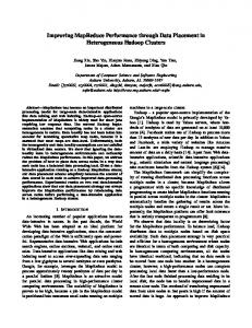
4. COORDINATING DATA AND COMPUTE OPERATIONS Our approach involves the explicit definition of data staging and offloading in a job script, followed by its decomposition and dependency setup. This infrastructure allows us to schedule and manage data jobs, resulting in better coordination with the computation. Figure 1 presents an overview of our architecture. Specification of I/O Activities: HPC users are already acclimatized to using sophisticated data transfer tools for their staging and offloading operations. Many times, these operations are embedded as part of the job script. However, these operations are not explicitly scheduled like compute jobs. As a first step towards the scheduling of data transfers, we have enabled the specification of these operations using “STAGEIN” and “STAGEOUT” directives. These data directives can be embedded within the job script much like resource manager directives (e.g., “#PBS” [25]). Such a specification allows a parser to extract the data staging/offloading commands to compose individual “data jobs” that can then be scheduled. In our implementation, we have instrumented a standard PBS job script [25]. Below is a simple example of a job script with data directives to stage-in data from the HPSS archival system [7] (using the hsi interface [11]) and to stage-out data (using scp). #PBS -N myjob #PBS -l nodes=128, walltime=12:00 #STAGEIN any parameters here #STAGEIN -retry 2 #STAGEIN hsi -q -A keytab -k my_keytab_file
End User
Machine Room Head Node Job Script
Compute Nodes
Job Queue
1. Stage Data 2. Compute Job 3. Offload Data
Planner
I/O Nodes
1 2 after 1 3 after 2
Data Queue Normal I/O access to staged data
Recovery Archive NFS access
Source copy of dataset accessed using: ftp, scp, GridFTP
Data Source
HSI access /home Staging
/scratch Parallel File System
Staging
Figure 1: Architecture for coordinated data and job orchestration. Also shown are various I/O activities such as staging, regular I/O operations and on-demand recovery from data sources in the machine-room and beyond. -l user “get /scratch/user/destination_file input_file” mpirun -np 128 ~/programs/myapp #STAGEOUT any parameters here #STAGEOUT scp /scratch/user/output/ user@destination_host:/home/user/
:
Of course, more complex staging and offloading logic can be constructed as long they are prefixed with the appropriate directive tags. Staging and offloading can also specify retry attempts with the “-retry” option. For a compute job several other parameters such as expected run time, priority, etc., are specified in the job script as resource manager directives. Similar parameters can also be specified for a data activity so they can be propagated to the resource manager. "Zero Charge" Data Transfer Queue: Fundamental to the scheduling of data staging and offloading activities is the treatment of these operations as “data jobs”. To achieve this, we propose establishing a separate queue (“dataxfer”) for data stage-in and stageout jobs (Figure 1). Doing so enables scheduler control over the staging and offloading activities. It is common practice for a supercomputer center to setup multiple queues to manage the diversity in user jobs. For instance, a computer center might setup different queues to handle all high-priority jobs, high throughput jobs (long running) or jobs requiring access to specific resources such as tapes. Multiple queues, in general, help service user jobs better. In our case, setting up separate queues for data and compute jobs is a step towards streamlining data operations by having them explicitly scheduled and managed. Further, it allows better coordination of staging and computing activities. In center operations, data transfers are not currently charged (the network and I/O bandwidth are not chargeable resources yet), which is also the reason why manual staging operations incur no cost. Storage allocations, on the other hand, are beginning to be charged. However, if this is so, it is a cost that users need to pay in any case. Now, the center can setup a “zero charge” data queue, to which staging and offloading jobs can be queued. The data queue should be scheduled based on the same scheduling policy used to manage the compute queue. For instance, if the compute queue uses priority-based scheduling, it makes sense for the data of the high priority job to arrive before the data for other jobs. Our ap-
proach enables this since we propagate parameters about data jobs from the job script to the resource manager. Finally, queuing up and scheduling data jobs separately also has the added benefit that these activities could be charged, if need be, in the future. To ensure that the dataxfer queue is not used by users for other computational jobs, we can limit access to the queue based on ACLs, which are supported by modern resource managers [24]. For instance, queue attributes such as host-based ACLs can be used to control the machines that can submit jobs to the dataxfer queue. Based on this, the scheduler on the head node can setup an ssh connection to a data job submission node (or I/O node) to submit stag-in and stage-out jobs to the dataxfer queue. Planning and Orchestration: We now have a way to specify and distinguish I/O activities such as staging and offloading alongside job scripts. Further, we have a dedicated data queue accepting transfer jobs. The next step is to devise a “plan” for execution. To this end, we have built a planner that accepts a PBS job script (shown above) and decomposes it into computing, staging and offloading jobs and their associated dependencies (see Figure 1). Let us say the compute, stage-in and stage-out jobs are stagin.pbs, compute.pbs and stageout.pbs, respectively. The stagin.pbs looks as follows: #PBS any parameters here retry looping construct here... hsi -q -A keytab -k my_keytab_file -l user “get /scratch/user/destination_file : input_file”
The stagout.pbs looks as follows: #PBS any parameters here scp /scratch/user/output/ user@destination_host:/home/user/
The compute.pbs looks as follows: #PBS -N myjob #PBS -l nodes=128, walltime=12:00 mpirun -np 128 ~/programs/myapp
The planner then sets up dependencies between these jobs and submits them to their respective queues using standard resource manager primitives. For example, an execution plan for the above three jobs might comprise the following steps. staginJobid=‘qsub -q dataxfer stagein.pbs‘ computeJobid=‘qsub -W depend=afterok:$staginJobid -q batch compute.pbs‘
qsub -W depend=afterok:$computeJobid -q dataxfer stageout.pbs
Here, we have used standard PBS primitives to set up dependencies and have used “qsub” to submit the jobs to the respective queues (batch and dataxfer). By explicitly specifying I/O activities and scheduling them along side compute jobs, we have ensured that the data will have arrived when the job is ready to be scheduled. Likewise, upon job completion, the offload data job is scheduled to transfer the data to its destination, thereby avoiding getting purged, waiting for manual intervention. Note, however, that our approach only ensures the timely initiation of the staging activity and cannot guarantee its completion due to other end-to-end issues (network vagaries and other storage issues). However, we do support retries of staging and offloading. If the staging activity failed, the compute job will not be scheduled. This way, the user, at least, does not waste his compute time waiting for data to become available. The scheduling of both data and compute operations poses the question: When should a job in the data queue be executed to enable “just-in-time” staging? This can be addressed by having estimates of queue wait times (using tools like NWS [35]) at the time of job submission and data transfer times, both of which are used as a measure to decide when to initiate staging. To start with, data transfer estimates can be specified by the user in much the same way estimated job run times are specified. Estimates of data transfer times can also be obtained between any two sites using transfer predictions (our earlier work [34]). This way, we can more closely tie the staging with the compute job. This also reduces the early stagein of the dataset and its associated pitfalls. However, this is beyond the scope of this paper and will be addressed in future work. Finally, to address the potential unavailability of prestaged data, due to storage system failure, before the job is scheduled, we have developed recovery stubs that perform data reconstruction if necessary (discussed in the next section). Since these recovery stubs are a means to cope with center failure, they will incur no cost to users’ allocated time. Thus, the coordinated scheduling helps improve center performance by mitigating the detrimental effects of failure.
5.
DATA RECOVERY AT NO COST TO ALLOCATED TIME
As mentioned earlier, recovery operations are necessary to reconstruct pre-staged data in the event of storage system failure before the job is scheduled. These operations are performed as periodic checks to ensure data availability for any given job. Further, recovery is performed as part of system management even before the job is scheduled. Therefore, its cost is not charged against the users’ compute time allocation. In the absence of reconstruction, user jobs are left to the mercy of traditional system recovery or put back in the queue for rescheduling. To start with, this mode of recovery is made feasible due to the transient nature of job data and the fact that they have immutable, persistent copies elsewhere. Next, many high-performance data transfer tools and protocols (such as hsi [11] and GridFTP [3]) support partial data retrieval, with which disjoint segments of missing file data—specified by pairs of start offset and extent—can be retrieved. Finally, the costs of network transfer is decreasing much faster than that of disk-to-disk copy. Collectively, these reasons enable and favor on-demand recovery. A staged job input data on the scratch parallel file system may have originated from the “/home” area or an HPSS archive [7] in the supercomputer center itself or from an end-user site. To achieve proactive data reconstruction, however, we need rich meta-
data about data source and transfer protocols used for staging. In addition, we need sophisticated recovery mechanisms built into parallel file systems. In the rest of this section, we will describe automatic recovery metadata extraction and the instrumentation of a parallel file system as an instance of how to achieve this on-demand data recovery.
5.1 Metadata: Recovery Hints To enable on-demand data recovery, we first propose to extend the parallel file system’s metadata with recovery information, which can be intelligently used to improve fault tolerance and data/resource availability. Staged input data has persistent origins. Source data locations, as well as information regarding the corresponding data movement protocols, can be recorded as optional recovery metadata (using the extended attributes feature) on file systems. For instance, the location can be specified as a uniform resource index (URI) of the dataset, comprised of the protocol, URL, port and path (e.g., “http://source1/StagedInput” or “gsiftp://mirror/StagedInput”). In addition to URIs, user credentials, such as GSI (Grid Security Infrastructure) certificates, needed to access the particular dataset from remote mirrors can also be included as metadata so that data recovery can be initiated on behalf of the user. Simple file system interface extensions (such as those using extended attributes) would allow the capture of this metadata. We have built mechanisms for the recovery metadata to be automatically stripped from a job submission script’s staging/offloading commands, facilitating transparent data recovery. One advantage of embedding such recovery-related information in file system metadata is that the description of a user job’s data “source” and “sink” becomes an integral part of the transient dataset on the supercomputer while it executes. This allows the file system to recover elegantly without manual intervention from the end users or significant code modification.
5.2 Data Reconstruction Architecture In this section, we present a prototype recovery manager. The prototype is based on the Lustre parallel file system [6], which is being adopted by several leadership-class supercomputers. A Lustre file system comprises of the following three key components: Client, MDS (MetaData Server) and OSS (Object Storage Server). Each OSS can be configured to host several OSTs (Object Storage Target) that manage the storage devices (e.g., RAID storage arrays). The reconstruction process is as follows. 1) Recovery hints about the staged data are extracted from the job script. Relevant recovery information for a dataset is required to be saved as recovery metadata in the Lustre file system. 2) The availability of staged data is periodically checked (i.e., check for OST failure). This is performed after staging and before job scheduling. 3) Data is reconstructed after OST failures. This involves finding spare OSTs to replace the failed ones, orchestrating the parallel reconstruction, fetching the lost data stripes from the data source, using recovery hints and ensuring the metadata map is up-to-date for future accesses to the dataset. Extended Metadata for Recovery Hints: As with most parallel file systems, Lustre maintains file metadata on the MDS as inodes. To store recovery metadata for a file, we have added a field in the file inode named “recov”, the value of which is a set of URIs indicating permanent copies of the file. The URI is a character string, specified by users during data staging. Maintaining this field requires little additional storage (less than 64 bytes) and minimal communication costs for each file. We have also developed two additional Lustre commands, namely lfs setrecov and lfs getrecov to set and retrieve the value of the “recov” field respectively, by
making use of existing Lustre system calls. I/O Node Failure Detection: To detect the failure of an OST, we use the corresponding Lustre feature with some extensions. Instead of checking the OSTs sequentially, we issue commands to check each OST in parallel. If no OST has failed, the probe returns quickly. Otherwise, we wait for a Lustre-prescribed timeout of 25 seconds. This way, we identify all failed OSTs at once. This check is performed from the head node, where the scheduler also runs. File Reconstruction: The first step towards reconstruction is to update the stripe information of the target file, which is maintained as part of the metadata. Each Lustre file f is striped in a round-robin fashion over a set of mf OSTs, with indices Tf = {t0 , t1 , . . . , tmf }. Let us suppose OST fi is found to have failed. We need to find another OST as a substitute from the stripe list, Tf . To sustain the performance of a striped file access, it is important to have a distinct set of OSTs for each file. Therefore, in our reconstruction, an OST that is not originally in Tf will take OST fi ’s position, whenever at least one such OST is available. More specifically, a list L of indices of all available OSTs is compared with Tf and an index ti′ is picked from the set L − Tf . We are able to achieve this, since Lustre has a global index for each OST. The new stripe list for the dataset is Tf′ = {t0 , t1 , . . . , ti−1 , ti′ , ti+1 , . . . , tmf }. When a client opens a Lustre file for the first time, it will obtain the stripe list from the MDS and create a local copy of the list, which it will use for subsequent read/write calls. In our reconstruction scheme, the client that locates the failed OST updates its local copy of the stripe and sends a message to the MDS to trigger an update of the master copy. The MDS associates a dirty bit with the file, indicating the availability of updated data to other clients. A more efficient method would be to let the MDS multicast a message to all clients that have opened the file, instructing them to update their local copies of the stripe list. This is left as future work. When the new stripe list Tf′ is generated and distributed, storage space needs to be allocated on OST ti′ for the data previously stored on OST ti . As an object-based file system [22], Lustre uses objects as storage containers on OSTs. When a file is created, the MDS selects a set of OSTs that the file will be striped on and creates an object on each one of them to store a part of the file. Each OST sends back the id of the object that it creates and the MDS collects the object ids as part of the stripe metadata. The recovery manager works in the same way, except that the MDS only creates an object in OST ti′ . The id of the object on the failed OST ti is replaced with the id of the object created on OST ti′ . The length of an object is variable [22] and, therefore, the amount of data to be patched is not required to be specified at the time of object creation. In order to patch data from a persistent copy and reconstruct the file, the recovery manager needs to know which specific byte ranges are missing. It obtains this information by generating an array of {of f set, size} pairs according to the total number of OSTs used by this file, mf , the position of the failed OST in the stripe list, i, and the stripe size, ssize. Stripe size refers to the number of data blocks. Each {of f set, size} pair specifies a chunk of data that is missing from the file. Given the round-robin striping pattern used by Lustre, it can be calculated that for a file with size f size, each size of the first k = f size mod ssize OSTs will have ⌈ fssize ⌉ stripes f size and each of the other OSTs will have ⌊ ssize ⌋ stripes. For each OST, it can be seen that in the jth pair, of f set = j × ssize, and in each pair except the last one, size = ssize. If the OST has the last stripe of the file, then size will be smaller in the last pair. The recovery manager then acquires the URIs to remote permanent copies of the file from the “recov” field of the file inode, as we described above. Then, it establishes a connection to the remote
data source, using the protocol specified in the URI, to patch each chunk of data in the array of {of f set, size} pairs. These are then written to the object on OST ti′ . We have built mechanisms so that the file reconstruction process can be conducted from the head node or from the individual OSS nodes (to exploit parallelism), depending on transfer tool and Lustre client availability. Patching Session: At the beginning of each patching operation, a session is established between the patching nodes (the head node or the individual OSS nodes) and the data source. Many data sources assume downloads occur in an interactive session that includes authentication, such as GridFTP [3] servers using UberFTP client [1] and HPSS [7] using hsi [11]. In our implementation, we use Expect [19], a tool specifically geared towards automating interactive applications, to establish and manage these interactive sessions. We used Expect so that authentications and subsequent partial retrieval requests to the data source can be performed over a single stateful session. This implementation mitigates the effects of authentication and connection establishment by amortizing these large, one-time costs over multiple partial file retrieval requests.
6. PERFORMANCE 6.1 Experimental Setup Our performance evaluation involves the following two steps. First, we assess the effect of storage node failures and its subsequent data reconstruction overhead on a real cluster using several local or remote data repositories as sources of data staging. Next, we use these benchmarking results in a simulation study that uses job traces, including job failure information, collected by large supercomputer centers to study the impact of our approach on the overall center performance in terms of average job wait time and wait time variances. Our testbed for evaluating the proposed data reconstruction approach is a 40-node cluster at Oak Ridge National Laboratory (ORNL). Each machine is equipped with a single 2.0GHz Intel Pentium 4 CPU, 768 MB of main memory, with a 10/100 Mb Ethernet interconnection. The operating system is Fedora Core 4 Linux with a Lustre-patched kernel (version 2.6.12.6) and the Lustre version is 1.4.7. Since our experiments focus on testing the server-side of Lustre, we have setup the majority of the the cluster nodes as I/O servers. More specifically, we assign 32 nodes to be OSSs, one node to be the MDS and one node to be the client. The client also doubles as the head node. In practice, such a group of Lustre servers will be able to support a fairly large cluster of 512-2048 compute nodes (with 16:1-64:1 ratios seen in contemporary supercomputers). We used three different data sources to patch pieces of a staged input file: (1) An NFS server at ORNL that resides outside the subnet of our testbed cluster (“Local NFS”) (2) an NFS server at North Carolina State University (“Remote NFS”) and (3) a GridFTP [4] server (“GridFTP”) with a PVFS [5] backend on the TeraGrid Linux cluster at ORNL, outside the Lab’s firewall, accessed through the UberFTP client interface [1].
6.2 Trace and Simulation Overview To evaluate the effect of our recovery mechanism on the overall performance of a supercomputing center, we perform tracedriven simulations based on the operational data released from Los Alamos National Laboratory [17]. This trace contains failure records for 24 HPC systems and job submission/completion records for 5 of them. Out of these 5 systems, system 20 is the largest one with 512 nodes and 4 CPUs per node. Therefore, we chose to base our simulations on this system. Two traces from sys-
6.3 Performance of Transparent Input Data Reconstruction As illustrated in Section 5, for each file in question, the reconstruction procedure can be divided into the following steps. 1) The failed OSTs are determined by querying the status of each OST. 2) The file stripe metadata is updated after replacing the failed OST with a new one. 3) The missing data is patched in from the source. This involves retrieving the URI information of the data source from the MDS, followed by fetching the missing data stripes from the source and subsequently patching the Lustre file to complete the reconstruction. These steps are executed sequentially and atomically as one transaction, with concurrent accesses, to the file in question, protected by file locking. The costs of the individual steps are independent of one another, i.e., the cost of reconstruction is precisely the sum of the costs of the steps. Below we discuss the overhead of each step in more detail. In the first step, all the OSTs are checked in parallel. The cost of this check grows with the number of OSTs due to the fact that more threads are needed to check the OSTs. Also, the metadata file containing the status of all OSTs will be larger, which increases the parsing time. This step induces negligible network traffic by sending small status checking messages. The timeout to determine if an OST has failed is the default value of 25 seconds in our experiments. Shorter timeouts might result in false positives. Figure 2 shows the results of benchmarking the cost of step 1 (detecting OST failures) when there are no such failures. In other words, this is the cost already observed in the majority of file accesses, where data unavailability is not an issue. In this group of tests, we varied the number of OSTs per I/O node (OSS), which in
0.30
Overhead(seconds)
tem 20 are used as input to our simulator. First is the node failure trace from system 20, which contains 2049 failure records over a period of 1349 days, each indicating specifications of a failure: the node number as well as the failure time and duration. Second is the job trace, which contains 489376 job submission and completion records over a period of 1073 days. Next, we explain how we couple the failure trace with the job trace. First of all, due to a lack of disk failure data, we focus on I/O node failures. These are failures that could not be automatically recovered using schemes such as RAID. Since the traces did not indicate whether I/O nodes were included or which nodes were I/O nodes, we assume all the 512 nodes are compute nodes and append additional nodes as I/O nodes. In most cluster systems, I/O nodes often share the same configuration as compute nodes (except for secondary storage). Therefore we extrapolate the failure statistics observed from the failure trace to these additional I/O nodes. More specifically, system 20’s node failure trace is used to calculate the average node failure rate and the average node failure repair time. We use those statistics to generate a set of failure events for each I/O node. Based on the job trace, we generate a set of job submission events, each of which contains the submission time, the execution time and the number of CPUs for a job. For parallel job scheduling, our simulator adopts the FIFO algorithm with backfilling, a popular choice in many supercomputing centers. The job trace, however, is devoid of staged data information (e.g., file size, stripe size, stripe count) for each job. To this end, we have obtained a snapshot of the Lustre scratch space from a production supercomputer center at ORNL. This staged data trace contains details of every file staged in the scratch parallel file system. We have calculated the distributions of file sizes, stripe sizes and stripe counts. We play these two traces together, randomly assigning staged data sizes to jobs, and study the average waiting times of jobs in Section 6.4.
1 OST/OSS 4 OST/OSS 16 OST/OSS
0.10 0.05 0.02 0.01
0.001 1
2
4
8
16
32
Number of storage nodes Figure 2: Cost of finding failed OSTs reality is configured by system administrators. High-end systems tend to have multiple OSTs per OSS, medium-sized or smaller clusters often choose to use local disks and have only one OST per OSS. From Figure 2, it can be seen that the overhead of step 1 is fairly small with a moderate number of OSTs. In most cases, the step 1 cost is under 0.05 seconds. However, this overhead grows sharply as the number of OSTs increases to 256 (16 OSTs on each of the 16 OSSs) and 512 (16 OSTs on each of the 32 OSSs). This can be attributed to the network congestion caused by the client communicating with a large number of OSTs in a short span. Note that the current upper limit of OSTs allowed by Lustre is 512, which incurs an overhead of 0.3 seconds, which is very small considering this is a one-time cost for input files only. 1
2
3
4
1
2
3
4
1
2
3
4
1
2
3
4
File size = 16MB, Stripe count = 4, Stripe size = 1MB
1
2
3
4
1
2
3
4
File size = 16MB, Stripe count = 4, Stripe size = 2MB
1
2
3
4
File size = 16MB, Stripe count = 4, Stripe size = 4MB
Figure 3: Round-robin striping over 4 OSTs The second recovery step has constant cost regardless of the number of OSTs as the only parties involved in this operation are the MDS and the client that initiates the file availability check (in our case, the head node). In our experiments, we also assessed this overhead and found it to be in the order of milliseconds. Further, this remains constant regardless of the number of OSSs/OSTs. The cost due to multiple MDS (normally two for Lustre) is negligible. The overhead of the third recovery step is expected to be the dominant factor in the reconstruction cost when OST failures do occur. Key factors contributing to this cost are the amount of data and the layout of missing data in the file. It is well known that non-contiguous access of data will result in lower performance than sequential accesses. The effect of data layout on missing data is more significant if sequential access devices such as tape drives
1MB chunk 2MB chunk 4MB chunk
Whole file staging in
64 16 4 1 0.25 128MB
256MB
512MB
1GB
2GB
1024 256
1MB stripe 2MB stripe 4MB stripe
Whole file staging in
64 16 4 1 0.25 128MB
256MB
File size
512MB
1GB
Patching cost(seconds)
256
Patching cost(seconds)
Patching cost(seconds)
1024
256
1MB chunk 2MB chunk 4MB chunk
Whole file staging in
64 16 4 1 0.25
2GB
128MB
256MB
File size
512MB
1GB
2GB
File size
(a) Remote NFS (b) Local NFS (c) GridFTP Figure 4: Patching costs for single OST failure from a stripe count 32. Filesize/32 is stored on each OST and that is the amount of data patched. Also shown is the cost of staging the entire file again, instead of just patching a single OST worth of data. 128
Patching cost(seconds)
are used at the remote data source. More specifically, factors that may affect patching cost include the size of each chunk of missing data, the distance between missing chunks, and the offset of the first missing chunk. Such a layout is mostly determined by the striping policy used by the file. To give an example, Figure 3 illustrates the different layout of missing chunks when OST 3 fails. The layout results from different striping parameters, such as the stripe width (called “stripe count” in Lustre terminology) and the stripe size. The shaded boxes indicate missing data stripes (chunks). We conducted multiple sets of experiments to test the data patching cost using a variety of file striping settings and data staging sources. Figures 4(a)-(c) show the first group of tests, one per data staging source (Remote NFS, Local NFS, and GridFTP). Here, we fixed the stripe count (stripe width) at 32 and increased the file size from 128MB to 2GB. Three popular stripe sizes were used with 1MB, 2MB, and 4MB chunks as the stripe unit, respectively. To inject a failure, one of the OSTs is manually disconnected so that 1/32 of the file data is missing. The y-axis measures the total patching time in log scale. For reference, a dotted line in each figure shows the time it takes to stage-in the whole file from the same data source (in the absence of our enhancements). We notice that the patching costs from NFS servers are considerably higher with small stripe sizes (e.g., 1MB). As illustrated in Figure 3, a smaller stripe size means the replacement OST will retrieve and write a larger number of non-contiguous data chunks, which results in higher I/O overhead. Interestingly, the patching costs from the GridFTP server remains nearly constant with different stripe sizes. The GridFTP server uses PVFS, which has better support than NFS for non-contiguous file accesses. Therefore, the time spent obtaining the non-contiguous chunks from the GridFTP server is less sensitive to smaller stripe sizes. However, both reconstructing from NFS and GridFTP utilize standard POSIX/Linux I/O system calls to seek in the file at the remote data server. In addition, there is also seek time to place the chunks on the OST. A more efficient method would be to directly rebuild a set of stripes on the native file system of an OST, which avoids the seek overhead that is combined with redundant read-ahead caching (of data between missing stripes) when rebuilding a file at the Lustre level. This, left as future work, should result in nearly uniform overhead approximating the lowest curve regardless of stripe size. Overall, we have found that the file patching cost scales well with increasing file sizes. For the NFS servers, the patching cost using 4MB stripes is about 1/32 of the entire-file staging cost. For the GridFTP server, however, the cost appears to be higher and less sensitive to the stripe size range we considered. The reason is that GridFTP is tuned for bulk data transfers (GB range) using I/O on large chunks, preferably tens or hundreds of MBs [21]. Also, the GridFTP performance does improve more significantly, compared with other data sources, as the file size increases.
64
1MB chunk 2MB chunk 4MB chunk
32 16 8 4 2 1 128MB/4
256MB/8
512MB/16
1GB/32
File size/Stripe count Figure 5: Patching from local NFS. Stripe count increases with file size. One OST fails and its data is patched. Figures 5 and 6 demonstrate the patching costs with different stripe counts. In Figure, 5 we increase the stripe count at the same rate as the file size to show how the patching cost from the local NFS server varies. The amount of missing data due to an OST 1 failure is stripe_count × f ile_size. Therefore, we patch the same amount of data for each point in the figure. It can be seen that the patching cost grows as the file size reaches 512MB and remains constant thereafter. This is caused by the fact that missing chunks in a file are closer to each other with a smaller stripe count. Therefore, when one chunk is accessed from the NFS server, it is more likely for the following chunks to be read ahead into the server cache. With larger file sizes (512MB or more), distances between the missing chunks are larger as well. Hence, the server’s readahead has no effect. Figure 6 shows the results of fixing the stripe size at 4MB and using different stripe counts. Note that a stripe count of 1 means transferring the entire file. From this figure, we can see how the cost of reconstructing a certain file decreases as the file is striped over more OSTs.
6.4 Job Scheduling Simulation Results In this section, we describe our results obtained by using the reconstruction numbers as input to trace-driven simulation of job wait times. Our simulations compare system performance with and without the reconstruction mechanism for different stripe counts. We use two metrics to evaluate system performance: the mean value and standard deviation(“SD”) of wait times of jobs. The SD of wait times is vital to center users because it represents an expected level of service. With our approach, we expect to improve the SD of wait times by eliminating the difference in wait times of failure-afflicted jobs and other successful jobs. Without recon-
64 16 4 1 0.25 1
4
8
16
Patching cost(seconds)
Patching cost(seconds)
Patching cost(seconds)
256 MB file 512 MB file 1 GB file
256
256 MB file 512 MB file 1 GB file
256 64 16 4 1 0.25
32
1
4
Stripe count
8
16
256 MB file 512 MB file 1 GB file
256 64 16 4 1 0.25
32
1
4
Stripe count
(a) Patching from remote NFS server
8
16
32
Stripe count
(b) Patching from local NFS server
(c) Patching from GridFTP server
w. reconstruction w/o reconstruction no failure
35000 30000 25000 20000 15000 10000 5000 0 4
8
16
32
SD of wait times(seconds)
Mean wait time(seconds)
Figure 6: Patching costs with stripe size 4MB 40000
100000
w. reconstruction w/o reconstruction no failure
80000 60000 40000 20000 0 4
8
16
32
(a) Original trace, mean wait time for all jobs
(b) Original trace, standard deviation (SD) for wait time of all jobs SD of wait times(seconds)
Stripe count
Mean wait time(seconds)
Stripe count
1e+06 100000 10000 1000 100 10 w. reconstruction w/o reconstruction
1 4
8
16
32
Stripe count
(c) Original trace, mean wait time for affected jobs
1e+06 100000 10000 1000 100 10 w. reconstruction w/o reconstruction
1 4
8
16
32
Stripe count
(d) Original trace, standard deviation (SD) for wait time of affected jobs
Figure 7: Simulation results with the original trace. Zero-wait jobs are omitted. struction, jobs encountering failure would be re-queued at the end of the queue. On the other hand, with our reconstruction, jobs that encounter an I/O node failure would only spend the cost of reconstruction as additional wait time. Moreover, the reconstruction cost can be hidden by proactive and periodic checking of the status of OSTs that host a job’s data. Our first set of simulation tests use the original LANL system 20 job trace combined with the staged data trace (see Section 6.2). In our experiments, we have tested different strategies of assigning a pair of {f ile_size, stripe_size} values from the staged data trace to each job (from the LANL trace). These include using fixed values for all jobs, using larger file sizes and stripe sizes for longer running jobs, and randomly picking a pair of values for each job. However, we find no observable difference between the strategies. The reason being, file sizes and stripe sizes only impact the reconstruction cost, which is hidden from the affected job in most cases due to our approach of proactive checking of the file’s availability. Therefore, we show the results of using randomly assigned file sizes and stripe sizes. As for stripe counts in the staged data trace, we find that more than 90% of the files are striped across 4 OSTs, according to the ORNL scratch space trace we obtained. In our simulations, we chose 4, 8, 16 and 32 for the stripe count values. Figure 7 shows the simulation results using the LANL job trace. The job traces follow a binomial distribution of job wait times (i.e., many short and few very long jobs exist in the queue). To address
this, we filtered the trace to remove jobs that have a zero wait time under all test configurations. As can be seen from Figure 7, the higher the stripe count, the more OSTs the files are associated with, which means an OST failure will affect more jobs. This intuitive trend can be observed for the job schedule without reconstruction. With our new reconstruction mechanism, however, the mean value and SD of wait times of all jobs are not affected by the increase in the stripe count, indicating a scalable solution for potentially very large Lustre server groups. Further, our reconstruction me chanism achieves the same mean value and SD of wait times as the ideal values (without any OST failure) for all stripe count settings (as the two curves are on top of each other). The second pair of charts in Figure 7 show the mean value and SD of wait times for the failure-affected jobs. There are two kinds of affected jobs. First are the scheduled and running jobs that access datasets located on the failed I/O node. These are now interrupted by the failure. Since we do not support online recovery yet, they will be rescheduled. The second set of jobs are yet to be scheduled, but have job input data located on the failed I/O node. If no reconstruction were applied, these jobs would have been moved to the tail of the job queue, waiting for their next turn to be dispatched. With reconstruction, however, they are scheduled immediately. For these affected jobs, the gains due to our new recovery mechanism are significant. The mean wait times are reduced from hundreds of thousands of seconds to tens of seconds.
8000 6000 4000 2000 0 35
49
65
79
SD of wait times(seconds)
Mean wait time(seconds)
w. reconstruction w/o reconstruction
10000
50000
w. reconstruction w/o reconstruction
40000 30000 20000 10000 0 35
49
65
79
(a) 16 OSTs, mean wait time for all jobs under different system work load
(b) 16 OSTs, standard deviation (SD) of wait times of all jobs under different system work load SD of wait times(seconds)
System workload(percentage)
Mean wait time(seconds)
System workload(percentage)
1e+06 100000 10000 1000 100 10 w. reconstruction w/o reconstruction
1 35
49
65
79
System workload(percentage)
(c) 16 OSTs, mean wait time for affected jobs under different system work load
1e+06 100000 10000 1000 100 10 w. reconstruction w/o reconstruction
1 35
49
65
79
System workload(percentage)
(d) 16 OSTs, standard deviation (SD) of wait times of affected jobs under different system work load
Figure 8: Simulation results with varying system work load The figure indicates that the mean value and SD of wait times for the affected jobs increases as the stripe count increases from 4 to 32. As mentioned earlier, a higher stripe count results in more jobs being afflicted due to an OST failure. Of those, affected running jobs that wait longer contribute to the mean wait time more than the affected jobs that are yet to be scheduled. Also, Figure 7 indicates that the mean wait time of affected jobs is much shorter than that of the set of all jobs. However, the mean wait time of the affected jobs should be longer than that of the set of all jobs since they not only incur the same wait time as the normal jobs but they also need to wait for the recovery. One possible reason for these results is that the job submission and failure logs used for the simulation have some special properties that cause affected jobs to have short wait times. One thing to note is that the failure log used for the I/O nodes is correlated to CPU failures, which could have an unintended effect on simulation results. When failures occur in a supercomputing center, typically all or some nodes are shut down and the job queue may refuse new jobs. Therefore, the job submission behavior may be altered as a consequence of center management policies regarding failure handling. As a result, fewer jobs exist in the job log around the failure times recorded, causing short wait times. In our experiments with system 20’s job trace, we find that the system CPU utilization rate is only 35%. To test our mechanism under heavier system work loads, we constructed a series of concatenated job traces based on the original trace by shortening the time interval between job submissions. Figures 8(a)-(b) depict the results of the set of all jobs. These results indicate that as the system work load increases, the mean wait time and the standard deviation with our mechanism increases slower than without our mechanism. In other words, the benefit of applying our reconstruction mechanism will be even more significant with heavier system work loads. For the affected jobs shown in Figures 8(c)-(d), with heavier system work loads, more running jobs are interrupted by the failures. Consequently, they need much more time to be rescheduled, waiting in the longer queue. Thus, the mean wait time increases from
tens of seconds to hundreds of seconds for the affected jobs with reconstruction. However, for the affected jobs without reconstruction, since the base is huge (around 100,000 seconds), the increase is not visible on the curve.
7. CONCLUSION In this paper, we have identified the need to manage transient job input/output data efficiently and have assessed its direct impact on supercomputer center performance as we approach petascale environments. We have built techniques to schedule data jobs alongside their computational counterparts to allow them to be scheduled in a synergistic fashion. Further, we have proposed a novel way to reconstruct transient, job input data in the face of storage system failure. Our simulation study of job traces and staged data, supported by data recovery measurements from a real supercomputer, suggests that our technique reduces the average wait time of jobs in a center significantly. In particular, more significant benefits are seen for long jobs and as data is stored over a larger number of I/O nodes. From a user’s standpoint, our techniques help reduce the job turnaround time and enable the efficient use of the precious, allocated compute time. From a center’s standpoint, our techniques improve serviceability by reducing the rate of resubmissions due to storage system failure and data unavailability. Further, they enable the optimal use of center resources (e.g., precious scratch space) by the timely staging and offloading of job input and output data.
8. ACKNOWLEDGMENT This research is sponsored in part by the Laboratory Directed Research and Development Program of Oak Ridge National Laboratory (ORNL), managed by UT-Battelle, LLC for the U. S. Department of Energy under Contract No. DE-AC05-00OR22725. It is also supported by an ECPI Award under contract No. DEFG02-05ER25685, a DOE grant DE-FG02-05ER25664, an NSF Grant CCF-0621470 and through Xiaosong Ma’s joint appointment between NCSU and ORNL. In addition, we thank Stephen Scott,
Thomas Naughton and Anand Tikotekar for providing us access to the XTORC cluster and helping us with the setup. Further, we also thank Gary Grider from LANL for the release of operational data and for helping us understand the traces.
9.
REFERENCES
[1] Ncsa gridftp client. http://dims.ncsa.uiuc.edu/set/uberftp/index.html, 2006. [2] J. Bent, D. Thain, A. Arpaci-Dusseau, R. Arpaci-Dusseau, and M. Livny. Explicit control in a batch aware distributed file system. In Proceedings of the First USENIX/ACM Conference on Networked Systems Design and Implementation, March 2004. [3] J. Bester, I. Foster, C. Kesselman, J. Tedesco, and S. Tuecke. GASS: A data movement and access service for wide area computing systems. In Proceedings of the Sixth Workshop on I/O in Parallel and Distributed Systems, 1999. [4] J. Bester, I. Foster, C. Kesselman, J. Tedesco, and S. Tuecke. Gass: A data movement and access service for wide area computing systems. In Proceedings of the 6th Workshop on Input/Output in Parallel and Distributed Systems, 1999. [5] P. Carns, W. Ligon III, R. Ross, and R. Thakur. PVFS: A Parallel File System For Linux Clusters. In Proceedings of the 4th Annual Linux Showcase and Conference, 2000. [6] Cluster File Systems, Inc. Lustre: A scalable, high-performance file system. http://www.lustre.org/docs/whitepaper.pdf, 2002. [7] R.A. Coyne and R.W. Watson. The parallel i/o architecture of the high-performance storage system (hpss). In Proceedings of the IEEE MSS Symposium, 1995. [8] Directed acyclic graph manager. http://www.cs.wisc.edu/condor/dagman/. [9] J. Kubiatowicz et al. Oceanstore: An architecture for global-scale persistent storage. In the 9th International Conference on Architectural Support for Programming Languages and Operating Systems, 2000. [10] S. Ghemawat, H. Gobioff, and S. Leung. The Google file system. In Proceedings of the 19th Symposium on Operating Systems Principles, 2003. [11] M. Gleicher. HSI: Hierarchical storage interface for HPSS. http://www.hpss-collaboration.org/hpss/HSI/. [12] J. Gray. Greetings from a file system user. ˜ http://research.microsoft.com/ Gray/talks/Fast_2005.ppt, 2005. [13] J. Gray and C.V. Ingen. Empirical measurements of disk failure rates and error rates. Technical Report MSR-TR-2005-166, Microsoft, December 2005. [14] J. Gray and A. Szalay. Scientific data federation. In I. Foster and C. Kesselman, editors, The Grid 2: Blueprint for a New Computing Infrastructure, 2003. [15] C. Hsu and W. Feng. A power-aware run-time system for high-performance computing. In SC, 2005. [16] T. Kosar and M. Livny. Stork: Making data placement a first class citizen in the grid. In Proceedings of 24th IEEE International Conference on Distributed Computing Systems (ICDCS2004), 2004. [17] Los Alamos National Laboratory. Operational data to support and enable computer science research. http://institutes.lanl.gov/data/fdata/, 2006. [18] Oak Ridge National Laboratory. Resources - national center for computational sciences (nccs).
http://info.nccs.gov/resources/jaguar, June 2007. [19] D. Libes. The expect home page. http://expect.nist.gov/, 2006. [20] M. Litzkow, M. Livny, and M. Mutka. Condor - a hunter of idle workstations. In Proceedings of the 8th International Conference on Distributed Computing Systems, 1988. [21] X. Ma, S. Vazhkudai, V. Freeh, T. Simon, T. Yang, and S. L. Scott. Coupling prefix caching and collective downloads for remote data access. In Proceedings of the ACM International Conference on Supercomputing, 2006. [22] M. Mesnier, G. Ganger, and E. Riedel. Object-based storage. IEEE Communications Magazine, 41(8):84–90, 2003. [23] H. Meuer, E. Strohmaier, H. Simon, and J. Dongarra. 29th top500 list of worlds fastest supercomputers released. http://www.top500.org/news/2007/06/23/29th_top500_list_world_s_fastest_supercomputers_released, June 2007. [24] Cluster resources inc. http://www.clusterresources.com/, 2007. [25] OpenPBS. Portable batch system. http://www.openpbs.org/. [26] D. Patterson, G. Gibson, and R. Katz. A case for redundant arrays of inexpensive disks (RAID). In Proceedings of the ACM SIGMOD Conference, 1988. [27] J. Plank, M. Beck, W. Elwasif, T. Moore, M. Swany, and R. Wolski. The Internet Backplane Protocol: Storage in the network. In Proceedings of the Network Storage Symposium, 1999. [28] K Ranganathan and I Foster. Decoupling computation and data scheduling in distributed data-intensive applications. In Proceedings of the High Performance Distributed Computing Symposium, 2002. [29] A Romosan, D Rotem, A Shoshani, and D Wright. Co-scheduling of computation and data on computer clusters. In Proceedings of the 17th International Conference on Scientific and Statistical Database Management (SSDBM 2005), 2005. [30] F. Schmuck and R. Haskin. GPFS: a shared-disk file system for large computing clusters. In Proceedings of the First Conference on File and Storage Technologies, 2002. [31] A. Shoshani, A. Sim, and J. Gu. Storage resource managers: Essential components for the grid. In J. Nabrzyski, J. Schopf, and J. Weglarz, editors, Grid Resource Management: State of the Art and Future Trends, 2003. [32] D. Thain, J. Basney, S. Son, and M. Livny. The kangaroo approach to data movement on the grid. In Proceedings of Tenth IEEE Symposium on High Performance Distributed Computing, 2001. [33] Top500 supercomputer sites. http://www.top500.org/, June 2007. [34] S. Vazhkudai and J. Schopf. Predicting sporadic grid data transfers. In Proceedings of the 11th IEEE Int’l Symposium on High Performance Distributed Computing (HPDC-11), 2002. [35] R. Wolski. Dynamically forecasting network performance using the network weather service. Journal of Cluster Computing, 1, 1998.