based JPALS application and the enhancement of a selection algorithm called EXM (Executive Monitor). The EXM examines the pass/fail outputs of other.
Optimizing Channel Selection for the JPALS´ Land-based Integrity Monitor Michael Koenig, Jason Rife, Sam Pullen, Per Enge, Stanford University ABSTRACT
1.0
JPALS (Joint Precision Approach and Landing System) is a precision landing system that provides LAAS (Local Area Augmentation System) like capabilities in a military operating environment. This paper discusses the landbased JPALS application and the enhancement of a selection algorithm called EXM (Executive Monitor). The EXM examines the pass/fail outputs of other monitors to define a common set of data based on exclusion of detected satellite or receiver faults. Prior versions of the EXM used heuristic rather than optimal criteria. Using data collected from Stanford´s LAAS IMT prototype, we evaluated the EXM algorithms with an analysis tool called the JTEP (JLIM Test Platform), where JLIM stands for the JPALS Land-based Integrity Monitor. The VPL (Vertical Protection Limit) is a high-integrity estimation of the landing aircraft’s vertical positioning error. It is a function of satellite geometry, the number of receivers, and the quality of each satellite’s ranging signal. When the VPL is below the VAL (Vertical Alarm Limit) the landing system is available. Our paper shows that an EXM decision method based on minimizing the VPL provides greater availability than previously achieved.
JPALS (Joint Precision Approach and Landing System) is a GPS landing system which provides LAAS (Local Area Augmentation System)-like precision approach and landing capabilities in a military environment. This paper discusses the development of a specific integrity monitor called the Executive Monitor (EXM) for land-based JPALS. This integrity monitoring capability is generally referred to as the JLIM (JPALS Land-based Integrity Monitor).
The traditional method of defining a common set by maximizing the number of receivers is less complex to code and less computationally demanding than the VPL based method. However, our results show the VPL method provides better availability performance with sufficient computational efficiency to enable real-time operation. To establish the performance benefits of the VPL-based method, this paper presents two analyses. The first details a comparison of EXM decision logic for the all-in-view satellite case. The second shows the robustness of VPLbased algorithms to a degraded one-satellite out case. The degraded constellation reflects a user aircraft which is unable to track all the satellites, an even which may occur commonly in JPALS due to jamming, interference, or aerial maneuvers (obstruction).
INTRODUCTION
One of the subsystems of the JLIM is a function called the EXM (for Executive Monitoring logic). The responsibility of this function is to take as inputs the pass/fail outputs of other monitors and to determine what action should be taken. Primarily, the EXM will look at which receiver/satellite channels have been passed and decide what the best common set to proceed with is. A channel represents an individual receiver-satellite pairing, e.g., satellite 2 on receiver 1 constitutes one channel. The common set is the group of satellites viewed on more than one receiver that the EXM approves for navigation. In the past, little attention has been given to EXM logic, because for nominal operations, the details of the EXM implementation have little impact on availability. The case is different under stress conditions. With jamming, or with marginal satellite visibility, which may be the norm for JPALS deployment, the EXM algorithm can make a significant difference in availability. If the intention is to maximize availability, then it is feasible to define a common set algorithm based on an availability metric. Since VPL is compared to VAL (Vertical Alarm Limit) in the user aircraft to determine availability, we have devised a VPL based algorithm. Prior versions of the EXM would choose a common set based on using the maximum number of GPS receivers that have current and valid observations (pseudorange and carrierphase), along with valid ephemeris. Since this system’s availability is determined by the VPL and not by that of some heuristic value such as the number of receivers, it is logical to incorporate the VPL into the decision making monitors of the system, i.e. the EXM.
We will be comparing the performance results of different methods to see which method is optimal. Thus, we expand the domain of algorithms which will determine the common set as an output of the EXM. These algorithms include maximizing the number of receivers, maximizing the number of satellites, minimizing the VPL, and minimizing the VPL when there will be a discrepancy between the tracked satellites of the ground station and user aircraft. The focus of this paper is to devise a selection method for the EXM which will maximize the availability of the JLIM system. This paper is comprised of four main sections as follows: 1) understanding the JLIM and the EXM, 2) specifying the system’s objective, 3) devising algorithms to achieve those objections, and 4) analyzing the performance of those algorithms. JLIM AND EXM BACKGROUND
The JLIM is a comprehensive collection of subsystems which process incoming measurements to determine code-phase corrections and simultaneously provide sufficient integrity to the user. The JLIM Test Platform, which is being developed at Stanford University, is referred to as the JTEP, and provides a means to test the relative advantages of various monitoring algorithms and architectures. This testbed has evolved from the LAAS Integrity Monitoring Testbed (IMT) [1,2], which is a similar development tool for LAAS which was also developed at Stanford. The JTEP has been developed to improve upon and extend the capabilities of its predecessor. Additions include the ability to handle an arbitrary (but plural) number of receivers, various input data formats, and more than one frequency (L1 & L2). Also, the JTEP has been coded in Matlab instead of Ccode to allow for easier development across platforms and to incorporate Matlab’s embedded utility libraries. 2.1
JLIM in Detail
Our software system, the JTEP, runs in the Matlab programming environment using data which has been archived from the Stanford LAAS IMT. This setup uses three Novatel OEM4 GPS receivers positioned to minimize the spatial correlation. The details of this implementation have been well documented in [1,2]. We have processed one data set which is approximately two hours long collected in March, 2003. The JTEP is a software framework which enables the developer to apply various monitor algorithms to determine which one will meet the JPALS requirements on accuracy, integrity, continuity, and availability. This includes individual algorithms designed to detect specific failure modes as well as the overall architecture of the entire system using all the employed monitors. We apply
Rx
Rx Rx
- JTEP -
QMs
Smoothing
Aircraft Broadcast
2.0
this principle to our assessment of the EXM algorithms. Figure 1 shows a simplified version of the JTEP. The JTEP takes as input receiver data that has been saved to file, and processes this data using several Quality Monitors [1] (denoted QMs). Using the pass/fail flags of the QMs and the smoothing function as input, the EXM decides what is the best common set of receivers and satellites with which to proceed. This common set dictates which satellites will be used to calculate measurement corrections. These corrections are averaged across receivers and examined to determine if any of the resulting satellite’s corrections are too large or have too much dispersion within their set of receivers. If the corrections are deemed acceptable, they are then broadcast to the aircraft. If not, the EXM will attempt to find a new common set after excluding the offending channels. The exact reason for requiring a common set is described in the following section.
Common Set
Executive Monitor iteration
Corrections
Fail Average
Pass
Figure 1: JTEP Simplified Block Diagram
2.2
EXM in Detail
In order to make the EXM as efficient as possible so that channels are not discarded unnecessarily, we use the JTEP to test variations of the candidate algorithms. The purpose of EXM is to evaluate which channels have failed any number of monitors and determine a common set of receivers and satellites which are deemed healthy. Among other things, internal JTEP monitors look at signal-to-noise ratio (SQM), parity errors (DQM), or measurement-trend errors (MQM). It is EXM’s responsibility to determine which measurements are not affected by failures, and from this information, what is the maximum usable “common set” of channels. As our monitoring system invokes the redundancy of receivers and satellites to determine if there is a possible failure, there needs to be consistency across the information being compared, particularly in the B-Value calculation [1].
- SV/Rx Pairings SV1 SV2 SV3 SV4 SV5 SV6 SV7 SV8 SV9 SVx Rx1 Rx2 Rx3
+ + +
+ + +
+ + +
+ + +
+ + x
+ + -
+ + -
x + +
+ x +
-
+ Healthy X Unhealthy − Untracked
Figure 2: EXM Pass/Fail Matrix The B-Value calculation is used to verify the consistency of measurements across multiple reference receivers. The B-Value is determined by subtracting off the average correction for each receiver (over all satellites) to remove the receiver clock bias, and then making a comparison across receivers (for each satellite) to determine the consistency of each satellite correction across receivers. If a common set is not used, then the subtraction of the average correction will be influenced by using different satellites. Please refer to Appendix A for more detail. 2.3
Standard EXM Algorithm
The standard algorithm for common set selection involves an iterative process which starts with the maximum number of receivers and searches for the maximum number of satellites for those receivers. This algorithm finds the common set which uses the most number of receivers, and if more than one common set satisfies this condition, chooses between them the common set which uses the most satellites. If at least four satellites cannot be found for this set, the process repeats for each subset of receivers. The emphasis is upon using the most receivers even though it is possible that other common sets are superior with regard to system availability. Consider the case illustrated in Figure 2, with potential common sets shown in Table 1. In the figure, channels with failed QMs are denoted as (x) and channels passed by all QMs are denoted by as (+). In the situation of Figure 2, the standard EXM will select the three receiver common set (solid brown outline), which includes only four healthy satellites. By comparison, a two receiver common set (dashed blue outline) exists that includes seven healthy satellites. A common set is not required to be contiguous, that was to clearly present the concept in the figure. The standard EXM does not consider whether the orange or the blue common set configuration might result in better availability. The choice of the blue common set presents two problems: 1) with only four satellites there will likely be poor geometry in calculating a position solution, thus the VPL will be high and availability will be threatened, 2) if for any reason the
aircraft using the JLIM’s satellite corrections was unable to use any one of those satellites, there would only be three usable satellites remaining and the system would be unavailable. (Sensor augmented GPS and the possibility of using less than four satellites is not considered) Issue one reveals the traditional algorithm’s threat to availability while issue two evinces the threat to availability via a ground station to aircraft satellite discrepancy, which we refer to as a threat to robustness. To avoid such vulnerabilities it is appropriate to specify an algorithm for choosing a common set which departs from the traditional heuristic method (shown in Table 1) in favor of a more deterministic approach.
Order
# Rxs
Rx List
# SVs
SV List
1
3
{1, 2, 3}
4
{1-4}
2
2
{1, 2}
7
{1-7}
3
2
{1, 3}
5
{1-4, 9}
4
2
{2, 3}
5
{1-4, 8}
Table 1: EXM Common Set Preference for Figure 1 3.0
PERFORMANCE OBJECTIVES
The focus of our research has been to increase the usability of the JLIM landing system. There are different performance criteria which define the operation of this system, including: accuracy, integrity, continuity, and availability. Our paper focuses on increasing the availability, or, the amount of time that the landing system can be used by aircraft to land with a prescribed amount of safety. This section describes two performance objectives associated with availability. The first objective is availability under nominal conditions, and the second is availability given a degraded satellite constellation (to the aircraft). The objectives necessitate the VPL calculation, which operates on receiver and satellite sets; additional mathematical background concerning sets and notation is detailed in the appendix.
3.1
Availability
4.0
Ongoing development of the JTEP shows that the traditional algorithm of the EXM is sub-optimal towards providing availability; hence we have examined the effect of EXM algorithms on availability. A direct calculation of the VPL as a function of the common set is made and compared to the predetermined VAL, thus determining if the landing system is “available”. The VPL is calculated by considering the quality of each satellite’s measurements and weighting them when calculating the GDOP matrix and their influence on the calculation of the vertical position. The VPL equation is: VPL = k ffnd (R)
∑ (σ
2 s
⋅ H 32, s
)
Where R is the set of receivers, S is the set of satellites, σs denotes the quality of the range measurement from satellite s, H3,i denotes the vertical component of the H matrix. H and the weighting matrix w are given below, and G is the standard GPS geometry matrix.
(
H = GT ⋅ w ⋅ G ⎛ σ 12 ⎜ w=⎜ 0 ⎜⎜ 0 ⎝
0 % 0
)
−1
0 ⎞⎟ 0 ⎟ ⎟ σ n2 ⎟⎠
⋅ GT ⋅ w
3.2
(2)
−1
Availability ≡ [ VPL(R ,S) < VAL ]
(3)
(4)
Robustness
Robustness defines the ability of the system to operate under a stressed condition. Here that condition is the circumstance that not all of the satellites, for which the ground station calculates corrections, are usable by the aircraft. This is referred to as a satellite discrepancy. The impetus for examining robustness is the possibility the aircraft will be unable to track a satellite due to jamming, interference, or signal obstruction from the aircraft’s own surfaces. Availability can be optimized by minimizing VPL, but this is truly only valid at the ground station even though it is calculated as a projection to the aircraft; however, the ground station can’t presume to know which satellites the aircraft is tracking. Thus, a set of corrections which is optimal at the ground station may in fact be useless to the aircraft simply because it is tracking a deleteriously distinct set of satellites. For the purposes of this paper, achieving robustness means choosing a common set such that any one satellite can be omitted and the resulting VPL will still be less than the VAL. Robustness ≡ ∀(s ε S) [ VPL(R, S-s) < VAL ]
This section discusses how different algorithms can be used to optimize for different objectives. As mentioned, the two performance objectives are availability and robustness, and we have examined the following four algorithms to determine their ability to achieve those objectives. Some algorithms are inherently optimal towards the objectives, thus we examine the suboptimality of the others. The four algorithms are: 1) 2) 3) 4)
(1)
s∈S
(5)
EXM ALGORITHMS
Maximize the number of Receivers used Maximize the number of Satellites used Maximize the Availability Maximize the Robustness to 1 Satellite out
The following sections detail the motivations for using each algorithm. Section 5 shows a comparison of algorithms applied to our two-hour data set. 4.1
Maximizing Receivers
Since multiple receivers must be used to enable system redundancy, the traditional method of set selection is based upon using the maximum number of receivers, which for this implementation, is three. When satellites are plentiful (i.e. good GDOP), and reducing from three receivers down to two only allows an increase from 11 to 12 satellites, it is very likely that the calculated VPL would benefit more by using the larger number of receivers than from the larger number of satellites as this lower the kffmd. Additionally, the B-Value calculations (which are also broadcast along with the corrections) are improved by increasing the number of receivers. The standard algorithm for common set determination first maximizes receivers, and then compares satellite count to break ties. It maximizes the quantity ΓRx (Eq. 6) where χ is a particular common set out of all the common sets X, and χRx is the optimal set for this algorithm. ΓRx ( χ ) = 100 ⋅ R + S
(6)
= ArgMax{ ΓRx (χ ), χ ∈ Χ }
χ Rx
(7)
The possible values of ΓRX are summarized in Table 2.
ΓRx 1 Rx 2 Rxs 3 Rxs
3 SV too few SVs
4 SVs
… 11 SVs 12 SVs too few Rxs
204
…
211
212
304
…
311
312
Table 2: Valuation for Maximizing Receivers
- SV/Rx Pairings SV1 SV2 SV3 SV4 SV5 SV6 SV7 SV8 SV9 SVx
+ + + + + + + x + + + + + + + + + x + + + + x - - + + -
Rx1 Rx2 Rx3
Set χA
1234 1234 1234
Set χB
1234567 1234567 Not used
+ Healthy X Unhealthy − Untracked
Set χC
Set χD
Not used
12348 12348
12349 12349
Not used
Figure 3: EXM Pass/Fail Subsets 4.2
4.3
Maximizing Satellites
For a position and time fix a GPS system must use a minimum of four satellites. To achieve the accuracy required of a GPS based landing system, many more satellites must be used to lower the VPL to an acceptable level. Increasing the number of satellites affects the VPL by ideally improving the satellite geometry and lowering the VDOP. Additionally, since the receiver clock biases are estimated by the mean of the measurements of the set of healthy satellites (see Section 2.2), having a larger set of satellites creates a better (less noisy) estimate of this bias. Maintaining many satellites also secures the system from a satellite discrepancy which is the focus of the robustness algorithm. There is no quantification of robustness here, but the two methods are related along this mode of reasoning. The quantity ΓSV is shown is Equation 8, and the common set χSV (Eq. 9) is chosen to maximize this value. ΓSV (χ ) = R + 100 ⋅ S
(8)
= ArgMax{ ΓSV (χ ), χ ∈ Χ }
χ SV
(9)
The possible values of ΓSV are summarized in Table 3.
ΓSV 1 Rx 2 Rxs 3 Rxs
3 SV too few SVs
4 SVs
… 11 SVs 12 SVs too few Rxs
402
…
1102
1202
403
…
1103
1203
Table 3: Valuation for Maximizing Satellites
Maximizing Availability
The availability of the JLIM is determined by the VPL being less than the VAL, so the optimal method for maximizing availability is to minimize VPL. Maximizing receivers or satellites is not without reason or merit, but they are ultimately heuristic methods. The availability of our integrity monitoring system is driven by its ability to calculate a correction and declare, with confidence, that the resulting position error will not exceed a bound. It is not feasible to derive a table as for the methods of MaxRx and MaxSV as the VPL is specific to the satellite constellation. For each epoch the JTEP runs, and for each potential common set, the EXM must compile the geometry matrix and perform several matrix multiplications and an inversion. Figure 3 shows the potential common sets for the situation illustrated in Figure 2. In this case, with three reference receivers, the availability maximization algorithm need compare only four common sets, { χA, χB, χC, & χD }, thus four VPLs are calculated for this algorithm, one for each common set. Although straightforward and involving only four matrix inversions, there is a significant increase in complexity compared to the previous methods which use only modest arithmetic. The MaxAV algorithm will outperform all other methods (with respect to availability), but the cost is the computational expense from the matrix inversions. System availability is Boolean whereas VPL is not, thus ΓAV is defined as the reciprocal of VPL so a comparison of ΓAV’s can be done even if two VPLs are both below the VAL. Thus, (VPL1 < VPL2 ) → ( ΓAV, 1 > ΓAV, 2 ). Γ AV ( χ ) =
χ AV
VAL VPL( χ )
= ArgMax{ Γ AV (χ ), χ ∈ Χ }
(10) (11)
Maximizing Robustness to One Satellite Out
5.0
The approach of maximizing availability is taken one step further by optimizing the system for availability in the presence of a ground station to user aircraft satellite discrepancy. The algorithm to maximize robustness to a one-satellite-out scenario involves the VPL calculation used in the previous section, but also an iteration over every satellite tracked within each potential common set. Given the four subsets of Figure 3, we must calculate 21 VPLs, ( 4 + 7 + 5 + 5 = 21 ), and even more if there were more satellites tracked. This algorithm chooses the common set which has the smallest of the maximum VPLs when iterated over that set’s satellites. By using the common set found by this method, we can calculate an upper bound on the user aircraft’s VPL even if they are using one fewer satellite than the ground station. In Equation 12, Xs is set notation to describe the set of all common sets determined by removing one satellite s from the set of satellites S comprising common set χ. Χ s ≡ { ( χ − s) | s ∈ S }
{ ( )
ΓRB ( χ ) = ArgMin Γ AV χ s , χ s ∈ Χ s
χ RB
= ArgMax{ ΓRB ( χ ), χ ∈ Χ }
4.6
Summary of Methods
}
2.2
Max Rxs Max SVs Max AV Max RB
2 1.8 1.6 1.4
(14)
1 0.8 0
100
200
300
400
500
600
Epochs (2 Hz.)
ss
Ro bu
stn e
Av ai
la bi lit y
cia l
tif i
#SV
VPL
VPL1SV
Traditional Heuristic
Max Rxs
Most Rxs
?
?
?
Additional Heuristic
Max SVs Max AV Max RB
?
Most SVs
?
?
?
?
Lowest VPL
?
?
?
?
Lowest VPL1SV
Ar
#Rx
Maximum Robustness
For ΓAV, the VAL was set to be 10m. Figure 5 below shows that, aside from the first 100 epochs of data where the receivers are just beginning to track the satellites, the system would be available using any of the EXM methods, although their margins of safety can vary noticeably.
1.2
Method
Maximum Availability
Availability Results
(13)
The relative computational cost and maximized output of each of the four algorithms is depicted in Figure 4 below, where VPL1SV = ( VAL / ΓRB ). To analyze the relative performance of these cost functions, the JTEP is used to compile this table at every epoch of the evaluated data set. The availability and robustness results follow as time plots in the next section. Increasing Computational Expense
5.1
(12)
ΓRB (Eq. 13) is the maximum VPL (minimum ΓAV ) calculated over each of the one-satellite out sets (χs ) of χ. In Equation 14, χRB is the common set chosen because it resulted in the maximum robustness of all χ’s in X.
RESULTS
Using the JTEP the four algorithms were applied to the data to determine their respective common sets. The availability (ΓAV) and robustness (ΓAV) of each of the common sets were calculated and are presented in the following sections. First are the results when using the algorithms when there is not a discrepancy between the satellites tracked by the ground station and aircraft, this represents availability. Second are the results of those algorithms when there is such a discrepancy, representing robustness.
ΓAV
4.5
Figure 4: Table of Methods and Outputs
Figure 5: ΓAV vs. Time for EXM Algorithms As expected the MaxAV algorithm has the maximum value for ΓAV. The MaxRx case was noticeably worse than the MaxAV case, at times being more than 1 meter larger. The MaxSV, MaxAV, and MaxRB algorithms demonstrate significant oscillation as they are a consequence of the varying inclusion and exclusion of satellites, particularly low elevation satellites. The MaxRB algorithm often uses the same common set as the MaxSV case, thus those two VPL curves often overlap. It is not always the case that all four algorithms yield ΓAV’s above unity. In Figure 6 the full two hours of the data set are shown. And though the volatility of the curves obscure one another, it can be seen from the plot that the MaxAV method always yields the largest ΓAV, and so, remains above unity the most frequently.
5.2
2.2 Max Rxs Max SVs Max AV Max RB
2
Figure 8 below shows an even more pronounced distinction between the traditional method of maximizing receivers, and the new VPL based methods of MaxAV and MaxRB.
1.6 1.4
1.6
1.2
1.4
1
1.2 5000
10000
15000
Epochs (2 Hz.)
Figure 6: ΓAV vs. Time for EXM Algorithms (2 Hrs) In order to elucidate the distinction between the algorithms, the data has been reduced to the difference in the VPL of each method to the MaxAV algorithm. This frees the availability results from being dependent upon the VAL, and the results are shown in Table 3. VPL Difference (m)
0
MaxRx - MaxAV MaxSV - MaxAV MaxRB - MaxAV
75.5 30.1 79.9
(0-1] (1-2] (2-3] (3-4] 4+ 14.8 67.9 19.5
3.6 0.1 0.0
0.0 0.3 0.3
0.2 0.0 0.0
5.9 1.6 0.4
Table 3: Frequency, in %, of VPL difference between each method and MaxAV (as baseline) Figure 7 shows the latter portion of the data set, where there is significant variability, and it reduces the data to being either available or not available, as depicted using the form (ΓAV > 1). All four methods shows significant periods of unavailability, but the MaxAV method, by design, will have the least unavailability. The most unavailable of all the algorithms is the MaxRx method, providing further evidence that this method is hindering the landing system’s overall performance.
ΓAV > 1
Yes
1.1
1.2
0.8 0.6 0.4 0.2 0 0
100
200
300
400
500
600
Epochs (2 Hz.) Figure 8: ΓRB vs. Time for EXM Algorithms The data set being used began recording data immediately after the Stanford IMT’s receivers were powered on, and so there are few satellites that are initially tracked. This was also evident in the plots of the section 5.1 where the ΓAV values rose noticeably during the first few minutes of operation As a consequence of the paucity of satellites, the MaxRx method (which typically uses the least number satellites) can not afford to lose any of its few and precious satellites, or it will suffer a significant increase of its VPL, as is evident in the plot. The MaxSV algorithm, which had the worst ΓAV performance, is identical to the MaxRB in this plot. Since this method emphasizes satellites, it can often sustain the loss of one satellite and still perform reasonably well. A longer rendering of the data, in fact shows the two methods diverge shortly after the last epoch shown in this figure.
Max Rxs Max SVs Max AV Max RB
Even though the MaxAV method provided the best availability (and robustness is a similar concept), there is no provision that dictates having good availability ensures having good robustness. This is the reason for taking the EXM study one step further. Not only is the MaxAV algorithm’s robustness performance noticeably worse compared to the MaxRB algorithm, it is certainly more variable.
1.3
Finally, as expected, the MaxRB algorithm has the largest value of ΓRB per epoch and the overall best robustness performance. Although the MaxRB method is just shy of achieving a unity value of ΓRB (for the duration shown), comparatively, it is clearly the best performing method.
No 1
Max Rxs Max SVs Max AV Max RB
1
0.8 0
ΓRB
ΓAV
1.8
Robustness Results for One-satellite-out
Epochs (2 Hz.) Figure 7: System Availability
1.4
1.5 4 x 10
1.6
1.2
ΓRB
VPL1SV Difference (m)
Max Rxs Max SVs Max AV Max RB
1.4
MaxRx – MaxRB MaxSV – MaxRB MaxAV – MaxRB
1
0
(0-1] (1-2] (2-3] (3-4]
63.8 9.3 10.5 47.1 49.7 1.6 80.2 13.5 2.0
0.6 0 0.5
4+
0.5 15.3 0.1 1.5 0.0 3.8
Table 4: Frequency, in %, of VPL1SV difference between each method and MaxRB (as baseline)
0.8 0.6 0.4 0.2 0
5000
10000
15000
Epochs (2 Hz.)
Figure 9: ΓRB vs. Time for EXM Algorithms (2 Hrs) Figure 9 above shows the full two hours of the data set. Here the MaxRx method actually agrees (chooses the same common set) as the MaxRB for the duration of time between epochs 5,000 and 10,000. The true setback of using the MaxRx method is the sheer unpredictability of the results. The epochs beyond 10,000 show all the algorithms to be unable to provide a ΓRB above unity, but the figure below shows whether the system is robust or not for the epochs 1,000-5,000.
Table 4 shows the improvement towards robustness when the EXM algorithms optimizes for this metric. Especially evident is the paltry performance of the MaxRx method. In fact, over this data set, more than 15% of the time the MaxRx method chose a common set whose VPL would be more than four meters higher, in the worst case scenario, than the common set chosen by the MaxRB method. 5.3
Results Summary
The total percentage of time the system is available and robust is presented in the following table.
Yes
Method
Available
Robust
MaxRx
82.4 %
58.1 %
MaxSV
87.2 %
59.5 %
MaxAV
88.5 %
61.5 %
MaxRB
88.5 %
64.9 %
Table 5: System Availability and Robustness
ΓRB > 1
Max Rxs Max SVs Max AV Max RB
No 1000
2000
3000
4000
5000
Epochs (2 Hz.) Figure 10: System Robustness In figure 10 there are multiple instances when the methods other than MaxRB have lost their robustness. Although the MaxSV algorithm only has a short spurt of non-robustness, such frailty could render the landing system unusable for the period around that occurrence because it has caused a lack of continuity. That is, there must be a finite, uninterrupted amount of time that the aircraft can use the landing system to perform the approach and landing. To appreciate the benefit to robustness, the data has been reduced to the difference in the VPL1SV of each method to the MaxRB VPL1SV, and the results are shown in Table 4.
The low values are due to the b-curve quality antenna term in the VPL equation. The MaxAV and MaxRB methods demonstrate their optimality as expected. The MaxRB method had the same availability performance as the MaxAV method because of the dual usage of the VPL. Within the data set, when many satellites where available there was an exact agreement between the two methods, but the periods of satellite outages evince the distinction. These results have shown that the EXM’s traditional method of selecting a common set without considering the VPL will result in sub-optimal performance. 6.0
FUTURE WORK
This paper utilized a two-hour data set taken by the Stanford LAAS installation. To meaningfully assess the impact of EXM algorithms on performance, additional, non-correlated data sets must be processed. This analysis has focused on the single frequency effects of EXM set selection, but the JPALS’ JLIM will be dual frequency, thus the analysis must extend to consider both L1 and L2. This paper has only considered those monitors in the system up to the first application of the EXM, which is EXM1[1]. More monitors exist in the JLIM, and a full treatment of this material will include EXM2 as well.
7.0
CONCLUSIONS
The JPALS’ EXM decision logic is responsible for determining a common set of measurements which will ultimately be used to calculate satellite pseudorange corrections for a landing aircraft. There are many criteria that can be used to distinguish one common set of receivers and satellites from another, and traditionally that criterion has been to select a common set which uses the most number of receivers. Our paper has shown that this heuristic method does not provide the maximum achievable system availability. We have proposed and investigated two new, VPL-based decision algorithms for the EXM. These algorithms, emphasizing availability and robustness respectively, perform better than the previous heuristic algorithm. This is especially true for robustness or, availability during a ground station to aircraft satellite discrepancy. Furthermore, the algorithms’ computational complexity does not inhibit real-time operation of the system. And finally, we recommend that the JPALS’ EXM incorporate the new VPL-based algorithm and apply them as appropriate to the operating environment. When ideal circumstances exist, i.e. no jamming, no interference, and using level approaches, the MaxAV (maximum availability) algorithm should be used. If the landing system operator determines that there is a threat to the aircraft of not being able to use all satellites, the MaxRB (maximum robustness) algorithm should be used.
APPENDIX A This section details the b-values calculation. Using a matrix P of pseudo-ranges, with two receivers and three satellites, we first remove the receiver clock bias by subtracting the average pseudo-range for that receiver, dubbed ρ i , where |Sk| is the number of satellites on receiver k. The first example (α) uses only a few channels of information (for clarity), and shows the faultiness of using a non-common set. ⎛ ρ1,1 ⎜ P = ⎜ ρ 2,1 ⎜ − ⎝ α
ρi =
REFERENCES [1] M. Luo, et.al. “Development and Testing of the Stanford LAAS Ground Facility Prototype,” Proceedings of the ION 2000 National Technical Meeting. Anaheim, CA., Jan 26-28, 2000, pp. 210-219. [2] G. Xie, et.al., “Integrity Design and Updated Test Results for the Stanford LAAS Integrity Monitor Testbed,” Proceedings of the 57th ION Annual Meeting. Albuquerque ,N.M., June 11-13, 2001, pp. 681-693. [3] P. Misra and P. Enge, Global Positioning System: Signals, Measurement and Performance, Ganga-Jamuna Press, Lincoln, MA, 2001.
−
ρ 1,3 ⎞ ⎟ − ⎟ − ⎟⎠
(A1)
Si
∑ (ρ )
(A2)
i, j
j =1
The resulting bias free (from receiver clock) matrix is: ⎛ ρ1,1 − ρ 1 ⎜ PC = ⎜ ρ 2,1 − ρ 2 ⎜ − ⎝ α
ρ 1, 2 − ρ1 ρ 2, 2 − ρ 2
ρ1,3 − ρ1 ⎞
−
−
−
⎟ ⎟ ⎟ ⎠
(A3)
The b-value associated with receiver 1 and satellite 1 is:
(
b1α,1 = PCα,(1,1) − 12 PCα,(1,1) + PCα,( 2,1) = (ρ 1,1 − ρ1 ) − (ρ 2,1 − ρ 2 ) =
ACKNOWLEDGMENTS The authors would like to give thanks to many other people in the Stanford GPS research group for their advice and interest. Funding support for this research comes from the Department of Defense JPALS Program Office. The opinions discussed here are those of the authors and do not necessarily represent those of any mentioned agencies or corporations.
1 Si
ρ1,2 ρ 2, 2
)
(23 ρ1,1 − 12 ρ 2,1 ) − [(13 ρ1,2 − 12 ρ 2,2 ) − 13 ρ1,3 ]
(A4)
Having no consistency when subtracting the pseudoranges to the same satellite across two receivers, causes the problem, and is a result of the imbalanced coefficients. Furthermore, the pseudorange to satellite 3 is unpaired, thus any fault existing on satellite 3 will appear to be a fault on receiver 1. To counter this inconsistency we require the use of a common set. The second example (β) shows the distinction.
P
β
⎛ ρ 1,1 ⎜ = ⎜ ρ 2,1 ⎜ − ⎝
ρ1, 2 ρ 2, 2 −
ρ1,3 ⎞ ⎟ ρ 2 ,3 ⎟
(A5)
− ⎟⎠
And with the receiver bias removed, the matrix is:
β
PC
⎛ ρ 1,1 − ρ1 ⎜ = ⎜ ρ 2,1 − ρ 2 ⎜ − ⎝
ρ1, 2 − ρ 1 ρ 2, 2 − ρ 2
ρ 1,3 − ρ 1 ⎞ ⎟ ρ 2, 3 − ρ 2 ⎟
−
−
⎟ ⎠
(A6)
(
b1β,1 = PCβ,(1,1) − 12 PCβ,(1,1) + PCβ,( 2,1)
[
)
]
= (ρ 1,1 − ρ1 ) − 12 (ρ1,1 − ρ1 ) + (ρ 2,1 − ρ 2 ) =
1 3
(ρ1,1 − ρ 2,1 ) − 16 [(ρ1,2 − ρ 2,2 ) + (ρ1,3 − ρ 2,3 )]
(A7)
Using a common set means that any fault common to a receiver is non-apparent in the b-value, and the b-value is an accurate representation of a receiver fault. The complete matrix of b-values can be given as
Bβ =
1 ⎛ 1 − 1⎞ β ⎟ ⋅ Pc ⎜ 2 ⎜⎝ − 1 1⎟⎠
(A8)
We can also collapse the preceding correction for the receiver clock bias and represent the entire b-value matrix as the following. ⎛ Bβ = ⎜Ι ⎜ ⎝
R
−
1 R
⎞ β ⎟⋅ P ⎟ ⎠
⎛ 1 ⎞ ⋅⎜ Ι S − ⎟ ⎜ S ⎟⎠ ⎝
Thus we conclude:
{ f ( Χ ) } ≠ { f (χ A ), f (χ B ), f (χ C ), ...} An operation to do this can be defined as:
{f
+
( Χ ) } ≡ { f (χ )| χ
∈ Χ}
⎧ χ * , such that, ⎫ ⎪⎪ ⎪⎪ ArgMax{ f (χ ), χ ∈ Χ } = ⎨ f χ * ≥ f (χ ), ⎬ ⎪ ⎪ * ⎪⎩ χ ∈ Χ, χ ∈ Χ ⎪⎭
( )
Element Operations on Sets
When a common set A consists of the receivers Rx1, Rx2, and Rx3, and satellites SV1 through SV5, the following nomenclature applies:
R A − Rx1 = { Rx 2 , Rx 3 }
(B1)
RA ≡ { Rx1 , Rx2 , Rx3 }
(B2)
χA ≡
(B3)
(B13)
Set functions and element removal are used in the paper on satellites, but it is more concise to use receivers here. {R A − r | r ∈ R A } ≡ {{Rx 2 , Rx 3 }, {Rx1 , Rx 3 }, {Rx1 , Rx 2 }}
Since a common set, χA, determines both SA and RA, we can meaningfully write the term χA- Rx1 as:
Therefore, VPL ( χ A ) = VPL
(B12)
(A9)
Element removal from a list is given as:
RA , S A
(B11)
But since our usage of functions on sets is always accompanied by a minimization or maximization, we will just use the standard ArgMin and ArgMax notation.
APPENDIX B
S A ≡ { SV1 , SV2 , SV3 , SV4 , SV5 }
(B10)
(
RA , S A
)
(B4)
X is the set of all potential common sets.
Χ ≡ { χ A , χ B , ...}
χ A − Rx1 = R A , S A − Rx1 = {Rx 2 , Rx 3 }, S A
(B15)
A function which iteratively removes one receiver is: (B5)
{χ A − r | r ∈ R A } = { {Rx 2 , Rx3 }, S A , {Rx1 , Rx 2 }, S A
,...}
Functions Applied to Sets
Via the association between χA and RA, we can also write:
Using a function upon a set yields the following.
{χ A − r | r ∈ R A } = {χ A − r | r ∈ χ A }
{ f ( χ ) | χ ∈ Χ} = { f ( χ A ),
f ( χ B ), ... }
(B6)
{ f(X) } may not have a meaning. This is illustrated by:
Φ ≡ {0, π2 , π , 32π , 2π }
(B7)
{Cos (φ ) |φ ∈ Φ } = {Cos (0), Cos ( π2 ),...}
(B8)
{Cos (Φ )} = {Cos (0, π2 , π , 32π ,2π ) } = ?
(B9)
(B17)
Symbology for an Excluded Element Set of Subsets The set of all those common sets formed by removing one receiver, or removing one satellite from χA are defined as:. Χ RA ≡ {χ A − r | r ∈ χ A }
(B18)
Χ SA ≡ {χ A − s | s ∈ χ A }
(B19)
If we wanted to remove two distinct elements, we would use the following symbols. Χ RS A ≡ {χ A − r − s | ( r ∈ χ A ), ( s ∈ χ A )}
Χ RR A ≡ {χ A − r1 − r2 | ( r1 ≠ r2 ), ( r1 ∈ χ A ), ( r2 ∈ χ A )}
Χ SS A ≡ {χ A − s1 − s 2 | ( s1 ≠ s 2 ), ( s1 ∈ χ A ), ( s 2 ∈ χ A )}
Χ RR A turns out to be quite simple and is given below.
Χ RR A = { Rx1 , S A , Rx 2 , S A , Rx 3 , S A
}
(B23)
This is just a notion to summarize a combinatorial expression. Χ RR A simply equates to the sets you would get if you had to remove two different receivers at a time. Since there were only three receivers to start with, there are three possibilities as shown above.