Optimizing compilation of constraint handling rules in HAL

arXiv:cs/0408025v1 [cs.PL] 10 Aug 2004

Under consideration for publication in Theory and Practice of Logic Programming

1

Optimizing Compilation of Constraint Handling Rules in HAL∗ CHRISTIAN HOLZBAUR Dept. of Medical Cybernetics and Art. Intelligence, University of Vienna, Austria

MARIA GARCIA DE LA BANDA School of Computer Science & Software Engineering, Monash University, Australia

PETER J. STUCKEY, GREGORY J. DUCK NICTA Victoria Laboratory, Department of Computer Science & Software Engineering, University of Melbourne, Australia submitted 31 August 2002; revised 2 March 2004, 28 June 2004; accepted 9 August 2004

Abstract To appear in Theory and Practice of Logic Programming (TPLP). In this paper we discuss the optimizing compilation of Constraint Handling Rules (CHRs). CHRs are a multiheaded committed choice constraint language, commonly applied for writing incremental constraint solvers. CHRs are usually implemented as a language extension that compiles to the underlying language. In this paper we show how we can use different kinds of information in the compilation of CHRs in order to obtain access efficiency, and a better translation of the CHR rules into the underlying language, which in this case is HAL. The kinds of information used include the types, modes, determinism, functional dependencies and symmetries of the CHR constraints. We also show how to analyze CHR programs to determine this information about functional dependencies, symmetries and other kinds of information supporting optimizations.

1 Introduction Constraint handling rules (Fr¨ uhwirth 1998) (CHRs) are a very flexible formalism for writing incremental constraint solvers and other reactive systems. In effect, the rules define transitions from one constraint set to an equivalent constraint set. Transitions serve to simplify constraints and detect satisfiability and unsatisfiability. CHRs have been used extensively (see e.g. (Holzbaur and Fr¨ uhwirth 2000)). Efficient implementations have been available for many years in the languages SICStus Prolog and ECLi PSe , and implementations for other languages are appearing such as Java (JCK 2002) and HAL. In this paper we discuss how to improve the compilation of CHRs by using additional information derived either from declarations provided by the user or from the analysis of the constraint handling rules themselves. The major improvements ∗ A preliminary version of this paper appeared under the title “Optimizing Compilation of Constraint Handling Rules” in ICLP 2001, Cyprus, November 2001 (Holzbaur et al. 2001).

2

C. Holzbaur & M. Garc´ıa de la Banda & P.J. Stuckey & G.J. Duck

we discuss over previous work on CHR compilation (Holzbaur and Fr¨ uhwirth 2000) are: • general index structures which are specialized for the particular joins required in the CHR execution. Previous CHR compilation was restricted to two kinds of indexes: simple lists of constraints for given Name/Arity and lists indexed by the variables involved. For ground usage of CHRs this meant that only list indexes are used. • continuation optimization, where we use matching information from rules earlier in the execution to avoid matching later rules. • optimizations that take into account algebraic properties such as functional dependencies, symmetries and the set semantics of the constraints. We illustrate the advantages of the various optimizations experimentally on a number of small example programs in the HAL implementation of CHRs. We also discuss how the extra information required by HAL in defining CHRs (that is, type, mode and determinism information) is used to improve the execution. In part some of the motivation of this work revolves around a difference between CHRs in Prolog and in HAL. HAL is a typed language which does not (presently) support attributed variables. Prolog implementations of CHRs rely on the use of attributed variables to provide efficient indexing into the constraint store. Hence, we are critically interested in determining efficient index structures for storing constraints in the HAL implementation of CHRs. An important benefit of using specific index structures is that CHRs which are completely ground can still be efficiently indexed. This is not exploited in the current Prolog implementations. As some CHR solvers only use ground constraints this is an important issue. The remainder of the paper is organized as follows. In the next section we give preliminary definitions, including the operational semantics of constraint handling rules. In Section 3 we go through the basic steps involved in compiling a set of constraint handling rules, and see how we can make use of properties such as functional dependencies and symmetry and set semantics in improving this basic compilation. In Section 4 we show how we can improve the compilation of a set of CHRs by discovering properties of constraints by reasoning about the form of the rules defining them. In Section 5 we show how to infer the functional dependencies and symmetry information, used in Section 3, from a set of CHRs. In Section 6 we give our experimental results illustrating the advantages of the optimized compilation. Finally, in Section 7 we conclude.

2 Constraint Handling Rules and HAL Constraint Handling Rules manipulate a global multiset of primitive constraints, using multiset rewrite rules which can take three forms simplification

[name@] c1 , . . . , cn ⇐⇒ g | d1 , . . . , dm

propagation

[name@] c1 , . . . , cn =⇒ g | d1 , . . . , dm

simpagation

[name@] c1 , . . . , cl \ cl+1 , . . . , cn ⇐⇒ g | d1 , . . . , dm

Optimizing Compilation of Constraint Handling Rules in HAL

3

where name is an optional rule name, c1 , . . . , cn are CHR constraints, g is a conjunction of constraints from the underlying language, and d1 , . . . , dm is a conjunction of CHR constraints and constraints of the underlying language. The guard part g is optional. If omitted, it is equivalent to g ≡ true. The simplification rule states that given a constraint multiset {c′1 , . . . , c′n } and substitution θ matching the multiset {c1 , . . . , cn }, i.e. {c′1 , . . . , c′n } = θ({c1 , . . . , cn }), where the execution of θ(g) succeeds, then we can replace {c′1 , . . . , c′n } by multiset θ({d1 , . . . , dm }). The propagation rule states that, for a matching constraint multiset {c′1 , . . . , c′n } where θ(g) succeeds, we should add θ({d1 , . . . , dm }). The simpagation rules states that, given a matching constraint multiset {c′1 , . . . , c′n } where θ(g) succeeds, we can replace {c′l+1 , . . . , c′n } by θ({d1 , . . . , dm }). A CHR program is a sequence of CHRs. More formally the logical interpretation of the rules is as follows. Let x ¯ be the variables occurring in {c1 , . . . , cn }, and y¯ (resp. z¯) be the other variables occurring in the guard g (resp. rhs d1 , . . . , dm ) of the rule. We assume no variables not in x ¯ appear in both the guard and the rhs.1 The logical reading is simplification

∀¯ x(∃¯ y g) → (c1 ∧ · · · ∧ cn ↔ (∃¯ z d1 ∧ · · · ∧ dm ))

propagation

∀¯ x(∃¯ y g) → (c1 ∧ · · · ∧ cn → (∃¯ z d1 ∧ · · · ∧ dm ))

simpagation

∀¯ x(∃¯ y g) → (c1 ∧ · · · ∧ cn ↔ (∃¯ z c1 ∧ · · · ∧ cl ∧ d1 ∧ · · · ∧ dm ))

The operational semantics of CHRs exhaustively apply rules to the global multiset of constraints, being careful not to apply propagation rules twice on the same constraints (to avoid infinite propagation). For more details see e.g. (Abdennadher 1997). Although CHRs have a logical reading (see e.g. (Fr¨ uhwirth 1998)), and programmers are encouraged to write confluent CHR programs, there are applications where a predictable order of rule applications is important. Hence, the textual order of rules in the program is used to resolve rule applicability conflicts in favor of earlier rules. The operational semantics is a transition system on a triple hs, h, tiv of a set of (numbered) CHR constraints s, a conjunction of Herbrand constraints h, and a set of transitions applied, as well as a sequence of variables v. The logical reading of hs, h, tiv is as ∃¯ y (s ∧ h) where y¯ are the variables in the tuple not in v. Since the variable component v never changes we omit it for much of the presentation. The transitions are defined as follows: Given a rule numbered a and a tuple hs, h, tiv c1 , . . . , cn =⇒a g | d1 , . . . , dk , dk+1 , . . . , dm where d1 , . . . , dk are CHR literals and dk+1 , . . . , dm are Herbrand constraints, such xc1 = ci1 ∧ that there are numbered literals {c′i1 , . . . , c′in } ⊆ s where |= h → ∃¯ · · · ∧ cn = cin and there is no entry (i1 , . . . , in , a) in t then the transition can be performed to give new state hs∪{d1 , . . . , dk }, h∧dk+1 ∧· · ·∧dm , t∪{(i1 , . . . , in , a)}iv where the new literals in the first component are given new id numbers.

1

This allows us to more easily define the logical reading, we can always place a CHR in this form, by copying parts of the guard into the right hand side of the rule and renaming.

4

C. Holzbaur & M. Garc´ıa de la Banda & P.J. Stuckey & G.J. Duck The rule for simplification is simpler. Given a tuple hs, h, tiv and a rule c1 , . . . , cn ⇐⇒ g | d1 , . . . , dk , dk+1 , . . . , dm

xc1 = ci1 ∧· · ·∧cn = cin such that there are literals {c′i1 , . . . , c′in } ⊆ s where |= h → ∃¯ ′ ′ the resulting tuple is hs \ {ci1 , . . . , cin } ∪ {d1 , . . . , dk }, h ∧ dk+1 ∧ · · · ∧ dm , tiv . In this paper we focus on the implementation of CHRs in a programming language, such as HAL (Demoen et al. 1999), which requires programmers to provide type, mode and determinism information. A simple example of a HAL CHR program to compute the greatest common divisor of two positive numbers a and b (using the goal gcd(a), gcd(b)) is given below. :- module gcd. :- import int. :- chr constraint gcd/1. :- export pred gcd(int). :- mode gcd(in) is det. base @ gcd(0) true. pair @ gcd(N) \ gcd(M) M >= N | gcd(M-N).

(L1) (L2) (L3) (L4) (L5) (L6) (L7)

The first line (L1) states that the file defines the module gcd. Line (L2) imports the standard library module int which provides (ground) arithmetic and comparison predicates for the type int. Line (L3) declares the predicate gcd/1 to be implemented by CHRs. Line (L4) exports the CHR constraint gcd/1 which has one argument, an int. This is the type declaration for gcd/1. Line (L5) is an example of a mode of usage declaration. The CHR constraint gcd/1’s first argument has mode in meaning that it will be fixed (ground) when called. The second part of the declaration “is det” is a determinism statement. It indicates that gcd/1 always succeeds exactly once (for each separate call). For more details on types, modes and determinism see (Demoen et al. 1999; Somogyi et al. 1996). Lines (L6) and (L7) are the 2 CHRs defining the gcd/1 constraint. The first rule is a simplification rule. It states that a constraint of the form gcd(0) should be removed from the constraint store to ensure termination. The second rule is a simpagation rule. It states that given two different gcd/1 constraints in the store, such that one gcd(M) has a greater argument than the other gcd(N) we should remove the larger (the one after the \), and add a new gcd/1 constraint with argument M-N. Note that M-N is the result of the subtraction of integer N from M, not the term -(M,N) that would be created in Prolog. Together these rules mimic Euclid’s algorithm. The requirement of the HAL compiler to always have correct mode information means that CHR constraints can only have declared modes that do not change the instantiation state of their arguments,2 since the compiler will be unable to statically determine when rules fire. Hence for example legitimate modes are in, which means the argument is fixed at call time and return time, and oo, which means that the argument is initialized at call time, but nothing further is known, 2

They may actually change the instantiation state but this cannot be made visible to the mode system.

Optimizing Compilation of Constraint Handling Rules in HAL

5

and similarly at return time. The same restriction applies to dynamically scheduled goals in HAL (see (Demoen et al. 1999)).

3 Optimizing the basic compilation of CHRs Essentially, the execution of CHRs is as follows. Every time a new constraint (the active constraint ) is placed in the store, we search for a rule that can fire given this new constraint, i.e., a rule for which there is now a set of constraints that matches its left hand side. The first such rule (in the textual order they appear in the program) is fired. Given this scheme, the bulk of the execution time for a CHR c1 , . . . , cl [, \]cl+1 , . . . , cn

⇐⇒ =⇒

g | d1 , . . . , dm

is spent in determining partner constraints c′1 , . . . , c′i−1 , c′i+1 , . . . , c′n for an active constraint c′i to match the left hand side of the CHR. Hence, for each rule and each occurrence of a constraint, we are interested in generating efficient code for searching for partners that will cause the rule to fire. We will then link the code for each instance of a constraint together to form the entire program for the constraint. In this section, when applicable, we will show how different kinds of compile-time information can be used to improve the resulting code in the HAL version of CHRs.

3.1 Join Ordering The left hand side of a rule together with the guard defines a multi-way join with selections (the guard) that could be processed in many possible ways, starting from the active constraint. This problem has been extensively addressed in the database literature. However, most of this work is not applicable since in the database context they assume the existence of information on cardinality of relations (number of stored constraints) and selectivity of various attributes. Since we are dealing with a programming language we have no access to such information, nor reasonable approximations. Another important difference is that, often, we are only looking for the first possible join partner, rather than all. In the SICStus CHR version, the calculation of partner constraints is performed in textual order and guards are evaluated once all partners have been identified. In HAL we determine a best join order and guard scheduling using, in particular, mode information. Since we have no cardinality or selectivity information we will select a join ordering by using the number of unknown attributes in the join to estimate its cost. Functional dependencies are used to improve this estimate, by eliminating unknown attributes from consideration that are functionally defined by known attributes. Functional dependencies are represented as p(¯ x) :: S x where S ∪ {x} ⊆ x ¯ meaning that for constraint p fixing all the variables in S means there is at most one solution to the variable x. The function fdclose(F ixed,F Ds) closes a set of fixed variables F ixed under the finite set of functional dependencies F Ds. fdclose(F ixed,F Ds) is the least set F ⊇ F ixed such that for each (p(¯ x) :: S x) ∈

6

C. Holzbaur & M. Garc´ıa de la Banda & P.J. Stuckey & G.J. Duck

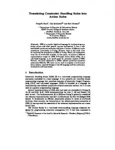
F Ds such that S ⊆ F then x ∈ F . Clearly the fixedpoint exists, since the operation is monotonic. We assume an initial set F ixed of known variables (which arises from the active constraint), together with the set of (as yet unprocessed) partner constraints and guards. The algorithm measure shown in Figure 1, takes as inputs the set F ixed, the sequence P artners of partner constraints in a particular order, the set F Ds of functional dependencies, and the set Guards of guards and returns the triple (score, Goal, Lookups). The score is an ordered pair representing the cost of the join for the particular order given by the n partner constraints in P artners. It is made up of the weighted sum (n − 1)w1 + (n − 2)w2 + · · ·+ 1wn−1 of the costs wi for each individual join with a partner constraint. The weighting encourages the cheapest joins to be earliest. The cost of joining the ith partner constraint to pre-join expression (the join of the active constraint plus the first (i − 1) partners), wi , is defined as the pair (u, f ): u is the number of arguments in the new partner which are unfixed before the join; and f is the negative of the number of arguments which are fixed in the pre-join expression. The motivation for this costing is based on the worst case size of the join, assuming each argument ranges over a domain of the same size s. In this case the number of join partners (tuples) in the partner constraint for each set of values for the pre-join expression is su , and there are sm−f tuples in the pre-join expression (where m is the total number of variables in the pre-join expression). The total number of tuples after the ith partner is joined are thus sm−f +u . The numbers hence represent the exponents of the join size, a kind of “degrees of freedom” measurement. The sum of the first components u gives the total size of the join. The role of the second component is to prefer orderings which keep the intermediate results smaller. We also take into account the selectivity of the guards we can schedule directly after the new partner. This is achieved via the selectivity(Guards) function which returns the sum of the selectivities of the guards Guards. The selectivity of a equational guard X = Y is 1 provided X and Y are both fixed, otherwise the selectivity is 0. An equation with both X and Y fixed immediately eliminates one degree of freedom (reduces the number of tuples by 1/s), hence the selectivity of 1. When one variable is not fixed, the guard does not remove any answers. For simplicity, the selectivity of other guards is considered to be 0.5 (as motivation, the constraint X > Y where X and Y can be considered to remove 0.5 degrees of freedom). The role of selectivity is to encourage the early scheduling of guards which are likely to fail. Goal gives the ordering of partner constraints and guards (with guards scheduled as early as possible). Finally, Lookups gives the queries. Queries will be made from partner constraints, where a variable name indicates a fixed value, and an underscore ( ) indicates an unfixed value. For example, query p(X, ,X,Y, ) indicates a search for p/5 constraints with a given value in the first, third, and fourth argument positions, the values in the first and third position being the same. The function schedule guards(F ,G) returns which guards in G can be scheduled given the fixed set of variables F . Here we see the usefulness of mode information

Optimizing Compilation of Constraint Handling Rules in HAL

7

measure(F ixed,P artners,F Ds,Guards) Lookups := ∅; score := (0, 0); sum := (0, 0) Goal := schedule guards(F ixed, Guards) Guards := Guards \ Goal while true if P artners = ∅ return (score, Goal, Lookups) let P artners ≡ p(¯ x), P artners1 P artners := P artners1 F Dp := {p(¯ x) :: f d ∈ F Ds} F ixedp := fdclose(F ixed, F Dp ) f¯ := x ¯ ∩ F ixedp F ixed := F ixed ∪ x ¯ GsEarly := schedule guards(F ixed, Guards) cost := (max(|¯ x \ f¯| − selectivity(GsEarly), 0), −|f¯| − selectivity(GsEarly)) score := score + sum + cost; sum := sum + cost ¯)} Lookups := Lookups ∪ {p((xi ∈ f¯ ? xi : ) | xi ∈ x Goal := Goal, p(¯ x), GsEarly; Guards := Guards \ GsEarly endwhile return (score, Goal, Lookups) schedule guards(F ,G) S := ∅ repeat G0 := G foreach g ∈ G if invars(g) ⊆ F S := S, g F := F ∪ outvars(g) G := Gs \ {g} until G0 = G return S

Fig. 1. Algorithm for evaluating join ordering

which allows us to schedule guards as early as possible. For simplicity, we treat mode information in the form of two functions: invars and outvars which return the set of input and output arguments of a guard procedure. We also assume that each guard has exactly one mode (it is straightforward to extend the approach to multiple modes and more complex instantiations). The schedule guards keeps adding guards to its output argument while they can be scheduled. The function measure works as follows: beginning from an empty goal, we first schedule all possible guards. We then schedule each of the partner constraints p(¯ x) in P artners in the order given, by determining the number of fixed (f¯) and unfixed (¯ x \ f¯) variables in the partner, and the selectivity of any guards that can be scheduled immediately afterwards. With this we calculate the cost pair for the join which is added into the score. The Goal is updated to add the join p(¯ x) followed by the guards that can be scheduled after it. When all partner joins are calculated the function returns.

8

C. Holzbaur & M. Garc´ıa de la Banda & P.J. Stuckey & G.J. Duck

Example 1 Consider the compilation of the rule: p(X,Y), q(Y,Z,T,U), flag, r(X,X,U) \ s(W) ==> W = U + 1, linear(Z) | p(Z,W).

for active constraint p(X,Y) and F ixed = {X, Y }. The individual costs calculated for each join in the left-to-right partner order illustrated in the rule are (2.5, −1.5), (0, 0), (0, −2), (0, −1) giving a total cost of (10, −11) together with goal q(Y,Z,T,U), W = U + 1, linear(Z), flag, r(X,X,U), s(W)

and lookups q(Y, , , ), flag, r(X,X,U), s(W). The best order has total cost (4.5, −7.5) resulting in goal flag, r(X,X,U), W = U + 1, s(W), q(Y,Z,T,U), linear(Z)

and lookups flag, r(X,X, ), s(W), q(Y, , ,U). For active constraint q(Y,Z,T,U), the best order has total cost (2, −8) resulting in goal W = U + 1, linear(Z), s(W), flag, p(X,Y), r(X,X,U)

and lookups s(W), flag, p( ,Y), r(X,X,U).  For rules with large-left-hand sides where examining all permutations is too expensive we can instead greedily search for a permutation of the partners that is likely to be cost effective. The current HAL implementation uses this method. In practice, both methods usually find the best ordering because the left-hand-sides of CHRs are generally small. 3.2 Index Selection Once join orderings have been selected, we must determine for each constraint a set of lookups of constraints of that form in the store. We then select an index or set of indexes for that constraint that will efficiently support the lookups required. Finally, we choose a data structure to implement each index. Mode information is crucial to the selection of index data structures. If the terms being indexed on are not ground, then we cannot use tree indexes since variable bindings will change the correct position of data.3 The current SICStus Prolog CHR implementation uses only two index mechanisms: Constraints for a given Functor/Arity are grouped, and variables shared between heads in a rule index the constraint store because matching constraints must correspondingly share a (attributed) variable. In the HAL CHR version, we put extra emphasis on indexes for ground data: The first step in this process is lookup reduction. Given a set of lookups for constraint p/k we reduce the number of lookups by using information about properties of p/k: 3

Currently HAL only supports CHRs with fixed arguments (although these might be variables from another (non-Herbrand) solver).

Optimizing Compilation of Constraint Handling Rules in HAL

9

• lookup generalization: rather than build specialized indexes for lookups that share variables we simply use more general indexes. Thus, we replace any lookup p(v1 , . . . , vk ) where vi and vj are the same variable by a lookup p(v1 , . . . , vj−1 , vj′ , vj+1 , . . . , vk ) where vj′ is a new variable. Of course, we must add an extra guard vi = vj for rules where we use generalized lookups. For example, the lookup r(X,X,U) can use the lookup for r(X,XX,U), followed by the guard X = XX. • functional dependency reduction: we can use functional dependencies to reduce the requirement for indexes. We can replace any lookup p(v1 , . . . , vk ) xj where there is a functional dependency p(x1 , . . . , xk ) :: {xi1 , . . . , xim } and vi1 , . . . , vim are fixed variables (i.e. not ) by the lookup p(v1 , . . . , vj−1 , , vj+1 , . . . , vk ). For example, consider the constraint bounds(X,L,U) which stores the lower L and upper U bounds for a constrained integer variable X. Given functional dependency bounds(X, L, U ) :: X L, the lookup bounds(X,L, ) can be replaced by bounds(X, , ). • symmetry reduction: if p/k is symmetric on arguments i and j we have two symmetric lookups p(v1 , . . . , vi , . . . , vj , . . . , vk ) and p(v1′ , . . . , vi′ , . . . , vj′ , . . . , vk′ ) where vl = vl′ for 1 ≤ l ≤ k, l 6= i, l 6= j and vi = vj′ and vj = vi′ then remove one of the symmetric lookups. For example, if eq/2 is symmetric the lookup eq( ,Y) can use the index for eq(X, ). We discuss how we generate functional dependency and symmetry information in Section 5. We can now choose the data structures for the indexes that support the remaining lookups. Normally, the index will return an iterator which iterates through the multiset of constraints that match the lookup. Conceptually, each index thus returns a list iterator of constraints matching the lookup. We can use functional dependencies to determine when this multiset can have at most one element. This is the case for a lookup p(v1 , . . . , vk ) with fixed variables vi1 , . . . , vim such that fdclose({xi1 , . . . , xim }, F Dp) ⊇ {x1 , . . . , xk } where F Dp are the functional dependencies for p/k, since in this case the functional dependencies ensure that for fixed vi1 , . . . , vim there can be at most one tuple in the constraint. For example, the lookup bounds(X, , ) returns at most one constraint given the functional dependencies: bounds(X, L, U ) :: X L and bounds(X, L, U ) :: X U. Since, in general, we may need to store multiple copies of identical constraints (CHR rules accept multisets rather than sets of constraints) each constraint needs to be stored with a unique identifier, called the constraint number. Code for the constraint will generate a new identifier for each new active constraint. Constraints that cannot have multiple copies stored at once are said to have set semantics (see section 4.4). In this case constraint numbers are not strictly necessary. Each index for p(v1 , . . . , vk ), where say the fixed variables are vi1 , . . . , vim , needs to support the following operations: :- pred p index init. :- mode p index init is det. :- pred p index insert(arg1, ..., argk, constraint num). :- mode p index insert(in, ..., in, in) is det.

10

C. Holzbaur & M. Garc´ıa de la Banda & P.J. Stuckey & G.J. Duck

:- pred p index delete(arg1, ..., argk, constraint num). :- mode p index delete(in, ..., in, in) is det. :- pred p index init iterator(argi1, ..., argim, iterator). :- mode p index init iterator(in, ..., in, out) is det.

for initializing a new index, inserting and deleting constraints from the index and returning an iterator over the index for a given lookup. Note that the constraint number is an important extra argument for index manipulation. In HAL indexes are stored in global variables, which are destructively updated for initialization, deletions and insertions. The compiler generates code for the predicates p insert constraint and p delete constraint which insert and delete the constraint p from each of the indexes in which it is involved. The current implementation supports three kinds of index structures: • A yesno global variable • A balanced 234 tree • An unsorted list (the default) By far the simplest index structure is a yesno global variable, which can have two states: a no state (meaning nothing is currently stored) or a yes(C) state, where C is the only constraint currently in the store. The compiler will generate a yesno index structure whenever it detects that it is not possible for multiple4 p/k constraints to exist in the store at once. This is the case whenever constraint p/k has set semantics (no identical copies) and has the functional dependencies p(¯ x) :: ∅ xi for xi ∈ x ¯ (all copies must be identical). An example is the constraint gcd/1 from the gcd example program in Section 2. Here the rule gcd(N) \ gcd(M) M >= N | gcd(M-N).

ensures one of the two gcd/2 constraints (one must be active) will be deleted. Therefore only one can ever actually be in the store at once, hence a yesno index structure may be used. If constraint p/k has set semantics and functional dependencies of the form p(x1 , . . . , xi , xi+1 , . . . , xk ) :: {x1 , . . . , xi } xj for all i < j ≤ k then the compiler will generate a balanced 234 tree index structure. In this case the constraint p/k can be thought of as defining a function from the key (x1 , . . . , xi ) to a value (xi+1 , . . . , xk ). For example, the constraint bounds(X,L,U) from the program in Figure A 1 in Appendix A has the functional dependencies bounds(X, L, U ) :: X L and bounds(X, L, U ) :: X U , hence the compiler builds a 234 tree index structure with X as the key, and the tuple (L,U) as the value. In addition, if the constraint p/k has set semantics, but has no functional dependency, then we can still use a tree index by treating the entire constraint as the key. For example, the constraint X != Y from the interval program in Appendix A has set semantics, 4

These constraints do not have to be identical.

Optimizing Compilation of Constraint Handling Rules in HAL

11

thus we can use a tree structure with (X,Y) as the key, and the empty set ∅ as the value. The big advantage of tree structures is O(log(n)) lookups whenever the key is fixed, compared with O(n) lookups for unsorted lists. Even if the key is only partially fixed there is still a potential for considerable benefit. Suppose that (X, Y ) is the key, then all keys of the form (X, ) will group together in the tree index because of HAL’s default ground term ordering. As a result, we can still do fast searches by pruning large sections of the tree that are not of interest. The same is not true for keys of the form ( , Y ) but we can sometimes use symmetric reduction to do the faster (Y, ) lookup instead. Example 2 The CHR constraint !=/2 defined by rules neqsym @ X != Y ==> Y != X. neqlower @ X != Y, bounds(X,VX,VX), bounds(Y,VX,UY) ==> bounds(Y,VX+1,UY). nequpper @ X != Y, bounds(X,VX,VX), bounds(Y,LY,VX) ==> bounds(Y,LY,VX-1).

has lookups !=(X, ) and !=( ,Y), and !=/(X,Y) and is known to be symmetric in its two arguments. We can remove the lookup !=( ,Y) in favor of the symmetric !=(Y, ), and then use a single balanced tree index for !=(X,Y) to store !=/2 constraints since this can also efficiently retrieve constraints of the form !=(X, ).  The advantage of using a tree is lost whenever there is a lookup which is not a prefix of the index. These lookups can be implemented using universal search over the tree, but this is particularly bad, since we need to construct a tree iterator, which is currently implemented as a tree to list conversion with high overhead. For simplicity, we currently do not use tree indices when at least one lookup is not a prefix of the key. Fortunately universal searches against the direction of the functional dependency are relatively rare in practice, and in the future implementations of universal searches might do away with the need for iterators altogether. The third and final type of index structure is an unsorted list. The advantage of a list index is fast O(1) insertions, but the disadvantages are slow O(n) lookups and deletions. However, if a constraint p/k is never deleted, and is often involved in universal searches, then a list is a logical choice for the index structure. 3.3 Code generation for individual occurrences of active constraints Once we have determined the join order for each rule and each active constraint, and the indexes available for each constraint, we are ready to generate code for each occurrence of the active constraint. Two kinds of searches for partners arise: A universal search iterates over all possible partners. This is required for propagation rules where the rule fires for each possible matching partner. An existential search looks for only the first possible set of matching partners. This is sufficient for simplification rules where the constraints found will be deleted. We can split the constraints appearing on the left-hand-side of any kind of rule into two sets: those that are deleted by the rule (Remove), and those that are not

12

C. Holzbaur & M. Garc´ıa de la Banda & P.J. Stuckey & G.J. Duck

bounds 4(X,L1,U1,CN1) :(bounds index exists iteration(X, ,L2,U2,CN2), CN1 != CN2 -> bounds remove constraint(X,L1,U1,CN1), bounds remove constraint(X,L2,U2,CN2), bounds(X,min(L1,L2),max(U1,U2)), %% RHS bounds 4 succ cont(X,L1,U1,CN1) ; bounds 4 fail cont(X,L1,U1,CN1) %% try next rule ).

Fig. 2. Existential search code for the fourth occurrence of a bounds/3 constraint (Keep). The partner search uses universal search behavior, up to and including the first constraint in the join which appears in Remove. From then on the search is existential. If the constraint has a functional dependency that ensures that there can be only one matching solution, we can replace universal search by existential search. For each partner constraint we need to choose an available index for finding the matching partners. Since we have no selectivity or cardinality information, we simply choose the index with the largest intersection with the lookup. Example 3 Consider the compilation of the 1st occurrence of the bounds/3 constraint in the rule (the fourth occurrence overall in the program in Figure A 1) intersect @ bounds(X,L1,U1),bounds(X,L2,U2) bounds(X,max(L1,L2),min(U1,U2)).

Since the active constraint is in Remove the entire search is existential. The compilation produces the code in Figure 2. The predicate bounds index exists iteration iterates non-deterministically through the bounds/3 constraints in the store using the index on the first argument. In the last 4 arguments it returns the 3 arguments of bounds/3 as well as a unique constraint number identifying the instance of the bounds/3 constraint.5 Note we check that the matching bounds/3 constraint has a different constraint number than the active constraint CN1 != CN2. The predicate bounds remove constraint removes the bounds/3 from the store. If the matching succeeds, then afterwards we call the success continuation bounds 4 succ cont (which will later be replaced by true), otherwise we call the failure continuation bounds 4 fail cont. The compilation for first occurrence of a bounds/3 constraint in the rule (the second occurrence overall) redundant @ bounds(X,L1,U1) \ bounds(X,L2,U2) L1 >= L2, U1 = L2, U1 %% Guard bounds remove constraint(X,L2,U2,CN1), %% remove matched constraint true %% RHS ; true %% rule did not apply ), (bounds alive(CN1) -> bounds 2 forall iterate(X,L1,U1,CN1,I1) ; true %% active has been deleted ).

Fig. 3. Universal search code for the second occurrence of a bounds/3 constraint The predicate bounds index init iterator, returns an iterator of bounds/3 constraints resulting from looking up the index. bounds iteration last and bounds iteration next respectively succeed if the iterator is finished and return values of the next bounds/3 (and its constraint number) as well as the new iterator. After the rule has fired, the predicate bounds alive checks that the active constraint has not been deleted as a consequence of executing the right-hand-side. If the active constraint is still alive, then we continue looking for more matchings. Note that for universal search we (presently) do not separate fail and success continuations.  Example 4 Consider the compilation of the 3rd occurrence of a gcd/1 constraint in the program in the introduction (the second occurrence in (L7)) which is to be removed. Since the active constraint is in Remove the entire search is existential. The compilation produces the code gcd 3 shown in Figure 4. The predicate gcd index exists iteration iterates non-deterministically through the gcd/1 constraints in the store using the index (on no arguments). It returns the value of the gcd/1 argument as well as its constraint number. Next, the guard is checked. Additionally, we check that the two gcd/1 constraints are in fact different by comparing their constraint numbers (CN1 != CN2). If a partner is found, the active constraint is removed from the store,

since the first argument must be known, but the compilation is more straightforward if it always returns all arguments.

14

C. Holzbaur & M. Garc´ıa de la Banda & P.J. Stuckey & G.J. Duck

gcd 2 forall iterate(N,CN1,I0) :gcd 3(M,CN1) :(gcd index exists iteration(N,CN2), gcd iteration last(I0), M >= N, CN1 != CN2 -> %% guard gcd insert constraint(N,CN1). gcd delete constraint(M,CN1), gcd 2 forall iterate(N,CN1,I0) :gcd(M-N), %% RHS gcd iteration next(I0,M,CN2,I1), gcd 3 succ cont(M,CN1) (M >= N, CN1 != CN2 -> %% guard ; gcd 3 fail cont(M,CN1) ). gcd delete constraint(M,CN2), gcd(M-N) %% RHS gcd 2(N,CN1) :; true %% rule did not apply gcd index init iterator(I0), ), gcd 2 forall iterate(N,CN1,I0), (gcd alive(CN1) -> gcd 2 cont(N,CN1). gcd 2 forall iterate(N,CN1,I1) ; true ).

Fig. 4. Code for existential partner search and universal partner search. and the body is called. Afterwards, the success continuation for this occurrence is called. If no partner is found the failure continuation is called. The compilation for second occurrence of a gcd/1 constraint (the first occurrence in (L7)) requires universal search for partners. The compilation produces the code gcd 2 shown in Figure 4. The predicate gcd index init iterator, returns an iterator of gcd/1 constraints resulting from looking up the index. Calls to gcd iteration last and gcd iteration next succeed if the iterator is finished and return values of the last and next gcd/1 constraint (and its constraint number) as well as the new iterator.  3.4 Joining the code generated for each constraint occurrence After generating the code for each individual occurrence, we must join it all together in one piece of code. The occurrences are ordered by textual occurrence except for simpagation rules where occurrences after the \ symbol are ordered earlier than those before the symbol (since they will then be deleted, thus reducing the number of constraints in the store). Let the order of occurrences be o1 , . . . , om . The simplest way to join the individual rule code for a constraint p/k is as follows: Code for p/k creates a new constraint number and calls the first occurrence of code p o1 /k + 1. The fail continuation for p oj /k + 1 is set to p oj+1 /k + 1. The success continuation for p oj /k + 1 is also set to p oj+1 /k + 1 unless the active constraint for this occurrence is in Remove in which case the success continuation is true, since the active constraint has been deleted. Example 5 For the gcd program the order of the occurrences is 1, 3, 2. The fail continuations simply reflect the order in which the occurrences are processed: gcd 1 continues to gcd 3 which continues to gcd 2 which continues to true. Clearly, the success continuation for occurrences 1 and 3 of gcd/1 are true since the active constraint

Optimizing Compilation of Constraint Handling Rules in HAL gcd(N) :new constraint number(CN1), gcd insert constraint(N,CN1), gcd 1(N,CN1). gcd 1(N,CN1) :(N = 0 -> %% Guard gcd delete constraint(N,CN1), true, %% RHS gcd 1 succ cont(N,CN1) ; gcd 1 fail cont(N,CN1)).

15

gcd 1 succ cont( , ). gcd 1 fail cont(N,CN1) :- gcd 3(N,CN1). gcd 3 succ cont( , ). gcd 3 fail cont(N,CN1) :- gcd 2(N,CN1). gcd 2 cont( , ).

Fig. 5. Initial code, code for first occurrence and continuation code for gcd is deleted. The continuation of gcd 2 is true since it is last. The remaining code for gcd/1 is given in Figure 5.6 

4 Improving CHR compilation In the previous section we have examined the basics steps for compiling CHRs taking advantage of type, mode, functional dependency and symmetries information. In this section we examine other kinds of optimizations that can be performed by analysis of the CHRs. 4.1 Continuation optimization We can improve the simple strategy for joining the code generated for each occurrence of a constraint by noticing correspondences between rule matchings for various occurrences. Suppose we have two consecutive occurrences with active constraints, partner constraints and guards given by the triples (p(¯ x), c, g) and (p(¯ y ), c′ , g ′ ) re′ ′ ¯ ¯ ¯V F spectively. Suppose we can prove that |= (¯ x = y¯ ∧ (∃y¯c ∧ g )) → ∃x¯ c ∧ g (where ∃ indicates the existential quantification of F for all its variables not in set V ). Then, anytime the first occurrence fails to match the second occurrence will also fail to match, since the store has not changed meanwhile. Hence, the fail continuation for the first occurrence can skip over the second occurrence. Example 6 Consider the following rules which manipulate bounds(X,L,U) constraints. ne @ bounds(X,L,U) ==> U >= L. red @ bounds(X,L1,U1) \ bounds(X,L2,U2) L1 >= L2, U1 X >= Y | ... r(A,B,C), p(C,D) ==> C < D | ...

The constraint X = C ∧Y = D∧(∃T q(Y, Y, X, T )∧X ≥ Y )∧(∃A, B, C r(A, B, C)∧ C < D) is clearly unsatisfiable and the success continuation of the first occurrence of p/2 can skip the second.  Currently the HAL CHR compiler performs very simple fail continuation optimization based on basic implication reasoning about identical constraints and true. Furthermore, because of some subtle complications arising from the implementation of universal searches, the current HAL CHR compiler restricts continuation optimization to existential searches. The difficulty stems from deciding if the head of the rule fires or not, which is information that this optimization relies upon. For the existential case there is no problem, since matching is already a mere semidet test. However a universal search may succeed multiple times, so some additional mechanism for recording the number of times a rule fires must be introduced. One possible solution is thread a counter through the code for the universal search, and count the number of times the search succeeds. If the counter is zero after the universal search code exists, then proceed with the fail continuation, otherwise proceed with the success continuation. This approach may be implemented in future versions of the compiler. 4.2 Late Storage The first action in processing a new active constraint is to add it to the store, so that when it fires, the store has already been updated. In practice, this is inefficient since it may quite often be immediately removed. We can delay the addition of the active constraint until just before executing a right-hand-side that does not delete the active constraint, and can affect the store (i.e., may make use of the CHR constraints in the store). Example 8 Consider the compilation of gcd/1. The first and third occurrences delete the active constraint. Thus, the new gcd/1 constraint need not be stored before they are executed. It is only required to be stored just before the code for the second occurrence. The call to gcd insert constraint can be moved to the beginning

Optimizing Compilation of Constraint Handling Rules in HAL

17

gcd(N) :new constraint number(CN1), gcd 1(N,CN1). gcd 1(N,CN1) :(N = 0 -> %% Guard true, %% RHS true %% success continuation ; gcd 3(N,CN1) %% fail continuation ). gcd 3(M,CN1) :(gcd index exists iteration(N,CN2), M >= N, CN1 != CN2 -> %% guard gcd delete constraint(M,CN1), gcd(M-N), %% RHS true %% success continuation ; gcd 2(M,CN1) %% fail continuation ). gcd 2(N,CN1) :gcd index init iterator(I0), gcd 2 forall iterate(N,CN1,I0). gcd 2 forall iterate(N,CN1,I0) :gcd iteration last(I0), gcd insert constraint(N,CN1). gcd 2 forall iterate(N,CN1,I0) :gcd iteration next(I0,M,CN2,I1), (M >= N, CN1 != CN2 -> %% guard gcd delete constraint(M,CN2), gcd insert constraint(N,CN1), %% late insert gcd(M-N) %% RHS ; true %% rule did not apply ), (gcd alive(CN1) -> gcd 2 forall iterate(N,CN1,I1) ; true ).

Fig. 6. Simplified code for gcd/1 with late storage of gcd 2, while the calls to gcd delete constraint in gcd 1 and gcd 3 can be removed. This simplifies the code for gcd/1 considerably, as illustrated in Figure 6.  The current implementation infers this information by a simple pre-analysis. We can consider a rule that does not delete the active constraint as rhs-affects-store if its right-hand-side calls a CHR constraint, or a local predicate which calls CHR constraints (directly or indirectly), or (to be safe) an external predicate which is not a library predicate. In future compiler implementations, when CHR constraints are allowed to have non-ground arguments, we must also ensure no left-hand-side

18

C. Holzbaur & M. Garc´ıa de la Banda & P.J. Stuckey & G.J. Duck

variables can ever be bound by the right-hand-side. This is because the CHR execution semantics dictate that whenever the instantiation state of a constraint changes, we must immediately run that constraint again as the active. However since the current implementation only supports ground CHR constraints, this issue is not yet relevant. Good late storage analysis is very important because most of the other analysis listed in this paper depends on it. Analysis for detecting set semantics, functional dependencies, never stored constraints and symmetry all rely on late storage information. 4.3 Never Stored A rule of the form c ⇐⇒ d1 , . . . , dm where c is a single constraint, always eliminates constraints of form c from the store. In particular if c is the most general form of the constraint p(x1 , . . . , xk ),7 and p/k does not need to be stored because of earlier occurrences of p/k in rhs-affects-store rules, then we don’t need to store this constraint at all. The advantage of neverstored information is that any rules involving p/k will only wake up when c is the active constraint. The current implementation searches for instances of never-stored rules and uses this information to avoid unnecessary joins, and to avoid building redundant index structures. Example 9 Consider a fixed/1 constraint which succeeds if its argument is a variable with equal lower and upper bounds, defined by the rules: bounds(X,V,V) \ fixed(X) true. fixed(X) fail.

Both rules delete the active fixed/1 constraint. Thus, there will never be a fixed/1 constraint in the store and hence an active bounds/3 constraint will never match the rule. Thus, the occurrence of bounds/3 in this rule will not be considered when compiling bounds/3.  4.4 Set semantics Although CHRs use a multiset semantics, often the constraints defined by CHRs have a set semantics. The current implementation detects two different forms of set semantics. Either the program rules ensure duplicate copies of constraints are always deleted or duplicate copies will not affect the behaviour of the program. The distinction between the two forms affects how the compiler takes advantage of this information, but in both cases set semantics allows us to choose more efficient index structures. 7

All arguments are pair-wise different variables.

Optimizing Compilation of Constraint Handling Rules in HAL

19

A constraint p/k has set semantics if there is a rule which explicitly removes duplicates of constraints. That is, if there exists a rule of the form p(x1 , . . . , xk ) [, \] p(y1 , . . . , yk ) ⇐⇒ g | d1 , . . . , dm ¯x¯∪¯y g which occurs before any rules require such that |= x1 = y1 ∧ · · · xk = yk → ∃ p/k to be stored. Example 10 The rule bounds(X,L1,U1) \ bounds(X,L2,U2) L1 >= L2, U2 >= U1 | true.

ensures that any new active bounds/3 constraint identical to one already in the store will be deleted (it also deletes other redundant bounds information). Since it occurs before any rules requiring bounds/3 to be stored the constraint has set semantics.  A constraint also has set semantics if all rules in which it appears behave the same even if duplicates are present. This is a very common case since CHRs are used to build constraint solvers which (by definition) should treat constraint multisets as sets. Thus, a constraint p/k also has set semantics if 1. there are no rules which can match two identical copies of p/k 2. there are no rules that delete a constraint p/k without deleting all identical copies. An exception is when the right-hand-side of such a rule always fails. 3. there are no rules with occurrences of p/k that can generate constraints (on the right-hand-side) which do not have set semantics. The current implementation uses a simple fixpoint analysis which can detect such constraints starting from the assumption that all constraints have set semantics. In each iteration a constraint which violates one of the rules above is deleted from the candidate set of those with set semantics. The iterations proceed until a fixpoint is reached. For constraints p/k having this form we can safely add a rule of the form p(x1 , . . . , xk ) \ p(x1 , . . . , xk ) ⇐⇒ true. This will avoid redundant work when duplicate constraints are added. We can also modify the index structures for this constraint to avoid the necessity of storing duplicates. Example 11 Consider a constraint eq/2 (for equality) defined by the CHR eq(X,Y),bounds(X,LX,UX),bounds(Y,LY,UY) ==> bounds(Y,LX,UX),bounds(X,LY,UY).

Then, since bounds/3 has set semantics, eq/2 also has set semantics. If we add the additional rule eq(X,Y), X != Y fail.

then eq/2 still has set semantics. Even though the additional rule might delete one copy only of the constraint eq/2, it does not matter because the rule leads to failure. 

20

C. Holzbaur & M. Garc´ıa de la Banda & P.J. Stuckey & G.J. Duck

Example 12 Adding the additional rule which deletes identical copies of constraints can improve the termination of the program. Consider the following rules which define symmetry for != constraints neqset @ X != Y \ X != Y true. neqsym @ X != Y ==> Y != X.

If we delete the rule neqset then rule neqsym is an infinite loop for any new !=/2 active constraint. However if !=/2 implicitly has set semantics, then we will automatically add the rule neqset, hence the program becomes terminating.  5 Determining Functional Dependencies and Symmetries In previous sections we have either explained how to determine the information used for an optimization (as in the case of rules which are rhs-affects-store) or assumed it was given by the user or inferred by the compiler in the usual way (as in type, mode and determinism). The only two exceptions (functional dependencies and symmetries) were delayed in order not to clutter the explanation of CHR compilation. The following two sections examine how to determine these two properties. 5.1 Functional Dependencies Functional dependencies occur frequently in CHRs since we encode functions using relations. Suppose p/k need not be stored before occurrences in a rule of the form p(x1 , . . . , xl , yl+1 , . . . , yk )[, \]p(x1 , . . . , xl , zl+1 , . . . , zk ) ⇐⇒ d1 , . . . , dm

(1)

where xi , 1 ≤ i ≤ l and yi , zi , l + 1 ≤ i ≤ k are distinct variables. This corresponds to the functional dependencies p(x1 , . . . , xk ) :: (x1 , . . . , xl ) xi , l + 1 ≤ i ≤ k. For example, the rule int of Example 6 illustrates the functional dependencies bounds(X, L, U ) :: X L and bounds(X, L, U ) :: X U . In addition, rule (1) deletes identical copies ensuring p/k has set semantics. Therefore there is at most one constraint in the store of the form p(x1 , . . . , xl , , . . . , ) at any time. Likewise, any constraint p/k that has a rule which deletes identical copies of constraints can also be thought of as having the functional dependency p(x1 , . . . , xk ) :: (x1 , . . . , xk ) ∅. Another common way functional dependencies are expressed in CHRs is by rules of the form p(x1 , . . . , xl , yl+1 , . . . , yk ), p(x1 , . . . , xl , zl+1 , . . . , zk ) =⇒ yl+1 = zl+1 , . . . yk = zk This leads to the same functional dependency as before, however it does not lead to set semantics behavior. We can detect more functional dependencies if we consider multiple rules of the same kind. For example, the rules p(x1 , . . . , xl , yl+1 , . . . , yk )[, \]p(x1 , . . . , xl , zl+1 , . . . , zk ) ⇐⇒ g1 |d1 , . . . , dm ′ ′ , . . . , zk′ ) ⇐⇒ g2 |d′1 , . . . , d′m′ p(x1 , . . . , xl , yl+1 , . . . , yk′ )[, \]p(x1 , . . . , xl , zl+1

Optimizing Compilation of Constraint Handling Rules in HAL

21

also lead to functional dependencies if |= (¯ y = y¯′ ∧ z¯ = z¯′ → (g1 ∨ g2 ) is provable. However because of the difficulty in solving disjunctions, the current analysis is limited to the case where g1 and g2 are primitive integer or real constraints (not conjunctions of other constraints). Example 13 The second rule for gcd/1 written twice illustrates the functional dependency gcd(N ) :: ∅ N since N = M ′ ∧ M = N ′ → (M ≥ N ∨ M ′ ≥ N ′ ) holds: gcd(N) \ gcd(M) M >= N | gcd(M - N). gcd(N’) \ gcd(M’) M’ >= N’ | gcd(M’ - N’).

Making use of this functional dependency for gcd/1 we can use a single global yesno integer value ($Gcd) to store the (at most one) gcd/1 constraint, we can replace the forall iteration by exists iteration, and remove the constraint numbers entirely. The resulting code (after unfolding) is gcd(X) :(X = 0 -> true ; (yes(N) = $Gcd, X >= N gcd(X-N) ; (yes(M) = $Gcd, M >= X $Gcd := yes(X), gcd(M-X) ; $Gcd := yes(X)))).

%% %% %% %% %% %% %%

occ 1: guard -> rhs occ 3: gcd index exists iteration, guard occ 3: rhs occ 2: gcd forall iterate, guard occ 2: gcd insert constraint occ 2: rhs late insert

 5.2 Symmetry Symmetry also occurs reasonably often in CHRs. There are multiple ways of detecting symmetries. A rule of the form p(x1 , x2 , . . . , xk ) =⇒ p(x2 , x1 , . . . , xk ) that occurs before any rule that requires p/k to be inserted induces a symmetry for constraint p(x1 , . . . , xk ) on x1 and x2 , providing that no rule eliminates p(x1 , x2 , . . . , xk ) and not p(x2 , x1 , . . . , xk ). Example 14 Consider a !=/2 constraint defined by the rules: neqset @ neqsym @ neqlower nequpper

X X @ @

!= Y != Y X != X !=

\ X != Y true. ==> Y != X. Y, bounds(X,VX,VX), bounds(Y,VX,UY) ==> bounds(Y,VX+1,UY). Y, bounds(X,VX,VX), bounds(Y,LY,VX) ==> bounds(Y,LY,VX-1).

the rule neqsym @ X != Y => Y != X illustrates the symmetry of !=/2 w.r.t. X and Y , since in addition no rule deletes a (non-duplicate) !=/2 constraint.  A constraint may be symmetric without a specific symmetry adding rule. The general case is complicated and, for brevity, we simply give examples.

22

C. Holzbaur & M. Garc´ıa de la Banda & P.J. Stuckey & G.J. Duck

Example 15 The rule in Example 11 and its rewriting with {X 7→ Y, Y 7→ X} are logically equivalent (they are variants illustrated by the reordering of the rule). eq(X,Y),bounds(X,LX,UX),bounds(Y,LY,UY) ==> bounds(Y,LX,UX),bounds(X,LY,UY). eq(Y,X),bounds(Y,LY,UY),bounds(X,LX,UX) ==> bounds(X,LY,UY),bounds(Y,LX,UX).

Hence, since this is the only rule for eq/2, the eq/2 constraint is symmetric.  Example 16 The following rules remove redundant inequalities: eq(X,Y) \ X = N | gcd(M-N).

The compiler uses this information to build a yesno index structure, since the functional dependency combined with set semantics implies that only one gcd(X) constraint can ever be in the store at one time. The next program, interval, is the most fruitful in terms of information discovered. The rules bounds(X,L1,U1) \ bounds(X,L2,U2) L1 >= L2, U2 >= U1 | true. bounds(X,L1,U1), bounds(X,L2,U2) bounds(X,max(L1,L2),min(U1,U2)). 8

See example 13 in Section 5.1

24

C. Holzbaur & M. Garc´ıa de la Banda & P.J. Stuckey & G.J. Duck

Table 1. Summary of the information extracted by the analysis phase of CHR compilation Program

Constraint

FD

gcd

gcd(X)

∅

interval interval interval interval interval

bounds(X,L,U) eq(X,Y) geq(X,Y) X != Y plus(X,Y,Z)

{X} — — — —

dfa

line(X,Y)

—

X L, U

Set

Sym

yes

—

yes yes yes yes yes

— — — {X, Y } —

yes

{X, Y }

leads to the the discovery of the set semantics of bounds/3 and the functional dependencies bounds(X, L, U ) : X L and bounds(X, L, U ) : X U . Therefore only one copy of the constraint bounds(X, , ) can ever be in the store at one time. The resulting structure for bounds/3 is a balanced 234 tree with (X) as the key and (L, U ) as the value. All of the other interval constraints at least have set semantics. Set semantics are inferred for constraints that behave the same even if multiple copies are stored. For example, the only rule involving the constraint eq/2 is equals @ eq(X,Y), bounds(X,LX,UX), bounds(Y,LY,UY) ==> bounds(Y,LX,UX), bounds(X,LY,UY).

Since bounds/3 has set semantics, then so has eq/2. The compiler uses this information to eliminate active eq/2 constraints that already occur in the store. Thus redundant work is avoided, and potentially the size of indexes is reduced. In addition symmetry on the constraint !=/2 is detected because of the symmetric rule neqsym @ X != Y ==> Y != X.

Because of the benefit with symmetric reduction, the compiler will choose a balanced 234 tree index for !=/2 with (X, Y ) as the key. Finally the dfa program turns out to be the least interesting in terms of information discovered. The only constraint with any useful attributes is line/2, which is symmetric and has set semantics. Again the compiler generates a balanced 234 tree index (for the same reasons as !=/2 in the interval program). All other constraints use the default unsorted list index structure. However, because of the large size of the heads of rules in the dfa program, the most important optimization is join ordering and early guard scheduling. The results gcd, interval and dfa are shown in Table 2, Table 3 and Table 4 respectively. All timings are the average over 20 runs on a 1200MHz AMD Athlon Processor with 1Gb of RAM running under Debian GNU Linux 3.0 with kernel

Optimizing Compilation of Constraint Handling Rules in HAL

25

Table 2. Execution times (ms) for various optimized versions of the gcd program Benchmark gcd gcd gcd gcd

Query

Orig

+yesno

+det

Hand

(5000000,3) (10000000,3) (50000000,3) (100000000,3)

1111 2314 12412 24891

976 2032 11093 22240

402 803 5095 10270

50 93 475 961

Table 3. Execution times (ms) for various optimized versions of the interval program Benchmark

Query

Orig

+tree

+det

+sym

+eq

interval interval interval interval interval interval interval interval

(12,1) (15,1) (20,1) (30,1) (12,2) (15,2) (20,2) (30,2)

389 1312 6077 73158 556 1824 8658 110224

138 382 1602 11728 184 532 2148 21950

126 355 1535 12537 167 471 1984 18799

67 172 693 4943 107 283 1135 8522

68 169 677 4916 69 167 669 5071

Table 4. Execution times (ms) for various optimized versions of the dfa program Benchmark dfa dfa dfa dfa dfa

Query

Prolog

+join

+treesym

+det

20 50 100 200 400

4987 69070 532278 too long too long

30 164 612 2804 13058

20 87 271 1525 7401

19 86 267 1536 7370

version 2.2.19, and are given in milliseconds. Any test taking more than 600000ms (10 minutes) is marked as “too long”. For gcd we first give times for the original output of the compiler Orig (uses a list index). In the version +yesno the list storage of constraints is replaced by a +yesno structure (using the functional dependency and set semantics). We can see a modest improvement here by just avoiding some overhead. Note that in Orig the list index for gcd/2 never grows more than one item in length anyway, so we do not

26

C. Holzbaur & M. Garc´ıa de la Banda & P.J. Stuckey & G.J. Duck

expect a significant improvement by replacing a singleton list with a yesno structure. In +det the determinism declarations of the compiled CHR code is altered to take into account the functional dependency. This is a low level optimization in which previously “nondeterministic” lookups can be declared semidet (can succeed at most once). Without this optimization they are declared cc nondet which means although they may succeed more than once we are interested only in the first solution. This produces faster executable code since deterministic (including semidet) code can be compiled in a simpler way than nondeterministic code. Finally Hand uses the hand optimized implementation of gcd/1 shown in Example 13. Here we see a considerable improvement purely from removing all of the overhead generated by the compiler (such as constraint numbers). We expect that future implementations of the compiler will be able to remove most of this excess overhead. The second experiment we show is interval in Table 3. The original code Orig uses list indexes for all constraints, version +tree is where the list index on bounds/3 has been replaced by a 234 tree index (using the functional dependency), +det where some cc nondet searches are correctly declared semidet, +sym where the list index on !=/2 has been replaced by a 234 tree index (because we can take advantage of symmetric reduction), and +eq where identical copies of set semantic constraints are deleted. Here we can see a significant improvement when the list index for bounds/3 is replaced by a 234 tree index. This is not surprising, since we are replacing O(n) lookups (for lists) with O(log(n)) lookups (for trees). Next the +det optimization provides a slight improvement in most cases. However for some unknown reason the test (30, 1) actually becomes slightly worse. Next the +sym lets us take advantage of symmetric reduction, which means we can choose a 234 tree index for the constraint !=/2. Again this provides a significant improvement. Finally the +eq optimization deletes identical copies of constraints before they run as the active constraint. The handling of set semantics is of considerable benefit when duplicate constraints are actually added, and doesn’t add significant overhead when there are no duplicate constraints, hence it seems worthwhile. The final example is the dfa program in Table 4. The code P rolog has the default join ordering and guard scheduling used by existing Prolog implementations of CHR compilers. Recall that this means guards are tested strictly after the join operation, hence the dreadful performance on a program with large rules, such as the dfa example. For the previous examples the default join ordering and the best join ordering coincide. Enabling join ordering and early guard scheduling (+join) produces a massive improvement in running time (dfa 100 is nearly 2000 times better). This highlights the importance of this optimization. Next +treesym turns on 234 tree indexes and symmetric lookup reduction for the line/2 constraint (without the symmetry lookup reduction, the compiler will not choose to use a 234 index because of a lookup line( , Y )). Once again we get a significant improvement. Finally in this case the +det optimization seems to produce a very slight improvement, if at all. Finally we remark that it is easy to optimize a very poor base implementation of CHRs. The HAL base implementation is highly efficient. The execution times of

Optimizing Compilation of Constraint Handling Rules in HAL

27

the Orig or P rolog columns are about an order of magnitude faster than CHRs in SICStus Prolog. See (Holzbaur et al. 2001) for more detail. 7 Conclusion and Future Work The core of compiling CHRs is a multi-way join compilation. But, unlike the usual database case, we have no information on the cardinality of relations and index selectivity. We show how to use type and mode information to compile efficient joins, and automatically utilize appropriate indexes for supporting the joins. We show how set semantics, functional dependencies and symmetries can improve this compilation process. We further investigate how, by analyzing the CHRs themselves we can find other opportunities for improving compilation, as well as determined functional dependencies, symmetries and other algebraic features of the CHR constraints. The prototype HAL CHR compiler which applies these techniques produces highly efficient CHR executables. Almost all of the optimizations considered in this paper are not specific to HAL, the optimizations that are not immediately applicable in a CHR compiler for Prolog are as follows. Mode information is not available for guards which means early guard scheduling may not be as effective, still assuming all variables are invars is safe and will account for most of the improvement. The determinism optimization +det in the experiments is not applicable since determinism declarations are not supported by Prolog systems. There is substantial scope for further optimization of CHRs. These include: more complicated lookups (for example range lookups on tree indexes), replacing propagation rules by equivalent simplification rules, common subexpression elimination, unfolding of CHRs, and determining invariant information for stored constraints. We plan to continue improving the HAL CHR compiler to take advantage of these possibilities. References Abdennadher, S. 1997. Operational semantics and confluence of constraint propagation rules. In Proceedings of the Third International Conference on Principles and Practice of Constraint Programming, G. Smolka, Ed. 252–266. Demoen, B., Garc´ıa de la Banda, M., Harvey, W., Marriott, K., and Stuckey, P. 1999. An overview of HAL. In Proceedings of the Fourth International Conference on Principles and Practices of Constraint Programming. 174–188. ¨ hwirth, T. 1998. Theory and practice of constraint handling rules. Journal of Logic Fru Programming 37, 1–3, 95–138. ¨ hwirth, T. 2000. Constraint handling rules, special issue. Journal Holzbaur, C. and Fru of Applied Artificial Intelligence 14, 4. Holzbaur, C., Stuckey, P., Garc´ıa de la Banda, M., and Jeffery, D. 2001. Optimizing compilation of constraint handling rules. In Logic Programming: Proceedings of the 17th International Conference, P. Codognet, Ed. LNCS. Springer-Verlag, 74–89. JCK 2002. JCK: Java constraint kit. http://www.pms.informatik.uni-muenchen.de/software/jack/index.html. Somogyi, Z., Henderson, F., and Conway, T. 1996. The execution algorithm of Mercury: an efficient purely declarative logic programming language. Journal of Logic Programming 29, 17–64.

28

C. Holzbaur & M. Garc´ıa de la Banda & P.J. Stuckey & G.J. Duck Appendix A Building a constraint solver in HAL using CHRs

The program in Figure A 1 defines a simple bounds propagation solver for integers using constraint handling rules. From a HAL perspective it is a solver module defining a solver on the type cint. Line (L3) is the type definition for the new type cint which is a wrapped integer. The integer is used as a variable number. The integer is wrapped so that we have a new type that we can (re-)define equality for.The type is exported abstractly hence its definition is not visible outside the module, thus restricting operations on cint to those in this module. Line (L4) is a re-instantiation declaration, which is required because we are going to treat cints in two ways. The reinst old declares a new instantiation cold (to be associated with the cint type) which is equivalent to “old” (i.e. a possibly non-ground term) outside the module, and equivalent to ground inside the module. We require this because outside the module we treat cints as bounds propagation solver variables, whereas inside the module they will be manipulated as wrapped integers (which are ground). Lines (L5) − (L6) give two common modes of usage for cints. Variable numbers (for new cints) are kept track of in a global integer counter VarNum. This is declared in line (L7) with its type int, and initial value (0). For any solver type we need to define two predicates init/1 which initializes a new variable and =/2 for equating two solver variables. Line (L8) is the predicate declaration for init/1 which is exported. Its mode is given in line (L9), the mode cno takes a new object and returns a cold object (old outside this module, and ground inside this module). Its definition in the next line simply returns the wrapped counter value, and increments the counter. The predicate must always succeed exactly once hence its determinism is det, but to pass determinism checking the call to bounds/3 is wrapped in an if-then-else (since the compiler cannot determine that it will not fail). The =/2 predicate is defined in line (L10) as export only, which makes it visible outside the module, but not visible inside the module. This is to avoid confusion with the equality on the internal view of cints which simply treats them as ground terms rather than integer variables. Its mode definition in line (L11) takes two cold cints as input and returns the same instantiation (the coo mode). It may fail, so the determinism is semidet. Note the definition of =/2 is made in terms of the non-exported constraint eq/2. Finally we arrive at our first constraint. Line (L12) defines an exported constraint bounds/3 which relates a cint to two ints. The mode declaration on line (L13) declares that the constraint must be invoked with an old cint and two ground integers. The CHR non empty is a simple propagation rule. Note the advantages of a typed language, the >= on the right hand side is integer comparison, not to be confused with the constraint >= defined on line (L16). The CHR redundant removes redundant bounds constraints. The CHR intersect replaces two bounds/3 constraints on the same variable by one. Note that bounds/3 occurs in many of the rules in the program not just the two defined immediately below its declaration. When compiling the module interval we can determine the functional dependencies: bounds(X, L, U ) :: X L and bounds(X, L, U ) :: X U , the symmetries eq(X, Y ) ≡ eq(Y, X), neq(X, Y ) ≡ neq(Y, X) and plus(X, Y, Z) ≡ plus(Y, X, Z) and that each of the CHR constraints has a set semantics. The lookups required for the program are (after reduction by functional dependencies): bounds(X, , ), eq(X,) , eq( , Y ), neq(X, Y ), neq(X,) , neq( , Y ), plus(X, , ), plus( , Y, ) and plus( , , Z). Symmetry eliminates the indexes eq( , Y ), neq( , Y ) and plus( , Y, ).

Optimizing Compilation of Constraint Handling Rules in HAL :::::::-

module interval. import int. export abstract typedef cint -> f(int). reinst old cold = ground. modedef cno -> (new -> cold). modedef coo -> (cold -> cold). VarNum glob var int = 0.

(L1) (L2) (L3) (L4) (L5) (L6) (L7)

:- export pred init(cint). (L8) :mode init(cno) is det. (L9) init(V) :- V = f($VarNum), $VarNum := $VarNum + 1, (bounds(V,-10000,10000) -> true ; error("not det.")). :- export only pred cint=cint. :mode coo=coo is semidet. X = Y :- eq(X,Y).

(L10) (L11)

:- export chrc bounds(cint,int,int). :mode bounds(coo,in,in) is semidet. non empty@ bounds(X,L,U) ==> U >= L. redundant@ bounds(X,L1,U1) \ bounds(X,L2,U2) L1 >= L2, U2 >= U1 | true. intersect@bounds(X,L1,U1), bounds(X,L2,U2) bounds(X,max(L1,L2),min(U1,U2)).

(L12) (L13)

:- chrc eq(cint,cint). :- mode eq(in,in) is semidet. equals @ eq(X,Y), bounds(X,LX,UX), bounds(Y,LY,UY) ==> bounds(Y,LX,UX),bounds(X,LY,UY).

(L14) (L15)

:- export chrc cint >= cint. :mode coo >= coo is semidet. geq @ X >= Y, bounds(X,LX,UX), bounds(Y,LY,UY) ==> bounds(Y,LX,UY), bounds(X,LX,UY).

(L16) (L17)

:- export :neqset @ neqsym @ neqlower@ nequpper@

chrc mode X != X != X != X !=

cint != cint. coo != coo is semidet. Y \ X != Y true. Y ==> Y != X. Y,bounds(X,VX,VX),bounds(Y,VX,UY)==>bounds(Y,VX+1,UY). Y,bounds(X,VX,VX),bounds(Y,LY,VX)==>bounds(Y,LY,VX-1).

:- export func cint + cint --> cint. :mode coo + coo --> oo is semidet. X + Y --> Z :- plus(X,Y,Z). :- chrc plus(cint,cint,cint). :- mode plus(in,in,in) is semidet. plus@ plus(X,Y,Z),bounds(X,LX,UX),bounds(Y,LY,UY),bounds(Z,LZ,UZ)==> bounds(X,LZ-UY,UZ-LY),bounds(Y,LZ-UX,UZ-LX),bounds(Z,LX+LY,UX+UY).

Fig. A 1. A simple integer bounds propagation solver using CHRs

29