Oct 22, 1992 - added random noise. An analysis of ... for radical-radical reactions, are obtained in com- ... and rate constants is often impossible to attain and.
Volume 98, Number 2, March-April 1993
Journal of Research of the National Institute of Standards and Technology [J. Res. Natl. Inst. Stand. Tcchnol. 98, 181 (1993)]
Optimizing Complex Kinetics Experiments Using Least-Squares Methods
Volume 98 A. Fahr, W. Braun, and M. J. Kurylo National Institute of Standards and Technology, Gaithersburg, MD 20899-0001
1.
Number 2
March-April 1993
Complex kinetic problems are generally modeled employing numerical integration routines. Our kinetics modeling program, Acuchcm, has been modified to fit rate constants and absorption coefficients generically to real or synthesized "laboratory data" via a leastsquares iterative procedure written for personal computers. To test the model and method of analysis the .self- and cross-combination reactions of HO2 and CH3O2 radicals of importance in atmospheric chemistry are examined. These radicals as well as other species absorb ultraviolet radiation. The resultant absorption signal is measured in the labo-
ratory and compared with a modeled signal to obtain the best-fit to various kinetic parameters. The modified program generates synthetic data with added random noise. An analysis of the synthetic data leads to an optimization of the experimental design and bestvalues for certain rate constants and absorption coefficients. Key words: CH3O3; computer modeling; complex gas phase kinetics; free radicals; HO2; least squares; optimization; simulated data. Accepted:
October 22, 1992
Introduction
Many rate constant determinations, particularly for radical-radical reactions, are obtained in complex kinetic systems in which more than one rate process and more than two species concentrations are involved. The kinetic processes can be first or second order or can be mixed. In such cases, an analytic relationship involving species concentrations and rate constants is often impossible to attain and numerical integration is required. If the measurements involve optical absorption, for example, an added complication of contributions to the signal from more than one species may arise. There are a number of modeling programs available to handle such complex systems but most are written for main-frame computers and few are capable of optimizing the fit of a given model to laboratory data by simultaneously adjusting a number of parameters [1]. To obtain a "best-fit" of the data to
the kinetic parameters the least squares procedure can be applied. While there is in principle only one least squares method [2,3], its application requires consideration of the conditional constraints relevant to each problem. These are sometimes referred to as the condition or adjustment equation (s). We describe in this paper the application of a computer program to a least squares fit that is applicable to any mechanism. However, the condition equations may be incomplete and the procedure for analyzing the fit of the parameters to the data should be examined carefully by the user. The kinetic modeling computer program, Acuchem [4] is now widely used. It has been modified in the present work to: 1) perform "Monte Carlo" simulations, and 2) to analyze synthetic data (with noise) via the least squares method and to yield a best fit 181
Volume 98, Number 2, March-April 1993
Journal of Research of the National Institute of Standards and Technology to various kinetic parameters within the constraints of the experiment. The program can also serve for the analysis of laboratory data as well an aid in the optimization of experimental design. The full program capabilities can be demonstrated through the application to the analysis of an important laboratory kinetics problem—which will be done in this paper. Here, the application of the program will be emphasized rather than its detailed construction. The details of the program will be published in near future. However, an interested reader wishing to implement methodology described here could request the program from authors. 2.
similar to the one described here are not fully automatic because operational decisions must be made. The possible variations in the analysis method are explored. 3.
Mechanism (Model)
The specific kinetic problem we investigate here consists of determining the cross-combination rate constant for two radicals of atmospheric interest, HO2 and CH3O2. Additional details of this system can be found elsewhere [5,6]. The experiments are complicated by overlapping absorptions from HO2 and CH3O2, uncertainties in absorption cross sections, and the inability to perform the experiment under first-order conditions. The objective of this paper is not resolving the disagreement concerning the correct values for absorption cross sections or rate constant for HO2 + CH3O2 but to demonstrate the application, capabilities, and limitations of our current kinetic modeling program. To do so, we have chosen the initial conditions and results of earlier studies of this system in our laboratory. Primarily, because conditions of other studies are not very clearly outlined in the literature [5,6]. There are three dominant reactions, two combination reactions and the cross-combination reaction. The initial radical concentrations (or rather their ratio) are in the range of previously used experimental values [5,6]. The units below in Eqs. (1) and (2) are cm^ molecule"' s"' for kx, molecules cm"^ for concentrations, nanometers for A, and 10"^" cm^ (base e) for absorption coefficient, &.
Procedure
The Acuchem modeling program requires an input file containing a kinetic mechanism with initialized rate constants and initial species concentrations. An output file is generated which lists the concentrations of all of the species on a preselected time grid, and can be displayed as a userdirected graph. We have written an additional program that converts the Acuchem output file into a synthetic "laboratory" data file. The name of each species is printed separately and the user can enter the contribution of each species in the composite "experimental" absorption signal. In normal practice, the synthetic data would be used to determine the sensitivity of the parameter(s) whose values are being sought to other measured variables. A new analysis program called Acufit has been devised. It reads the Acuchem input file, assumed to contain the correct mechanism or "model," and then either the synthetic "laboratory" or real laboratory data. This is fitted to the "model" in a prescribed way. Both rate constants and absorption coefficients (representing the contribution of each species to the signal) can be adjusted. An iterative adjustment procedure is employed. These problems are inherently nonlinear and one adjustment around initial "first guess values" (by taking only first derivatives) is usually not sufficient. Of course first guess values are necessary and, as long as they are not too divergent from the "correct" values, the iterations will converge (if a solution is possible, see below). Adjustments are made via solution of the "normal equations." Because the variancecovariance matrix is readily available, the quality of the fit can be assessed. Solving for all possible parameters in the system is usually not possible in that multiple (degenerate or near-degenerate) solutions can often fit the data equally well. Programs
H02 + H02^H202 + 02,
A:, = 1.86x10"'^
CH3O2 + CH3O2 -> products,
A:2 = 3.60x10"'^
HO2 + CH3O2 -> CH3O2H + O2,
h = 2.90 X10-'^
[H02]i) + [CH302})= 10.8 X 10'^
A (215)
[H02]n+[CH302]o= 11.8X 10'\
A(250) (1)
The parameters listed are used to synthesize a good surrogate to the "real" laboratory data, which can be used for test purposes. The objective here is to assess the optimum conditions for obtaining a best fit to the cross-combination rate constant fe. The rate constants ki and fc and the e's are best obtained in single component systems [7,8,9,10] containing only HO2 or CH3O2. Any complex experiment of this kind entails conditions that are characteristic of the experimental design. Those that apply to an earlier study from this laboratory [5] are given in Eq. (2). 182
Volume 98, Number 2, March-April 1993
Journal of Research of the National Institute of Standards and Technology concentrations (always assumed to be known) and the rate constants, ^i, kz, and ki taken as initial first estimates. Acufit also requires specification of the parameters (k's or e's) to be evaluated and their initial assignments. Parameters not to be evaluated (fixed) are held at their input values. Finally Acufit requests the value for the random (normally distributed) noise on the data and whether the noise distribution is to be always the same (unseeded) or randomly variable (seeded) from run to run. In the present study the "noise" or a applied to the data is taken to be independent of the signal level, common for most absorption experiments. Since the initial assignments for all of the parameters are similar to those used in the construction of the synthetic "laboratory" file, Acufit might return values very close to these, depending upon the entered level of noise. In most cases, however, the sums of residuals squared either increase with successive iterations or oscillate such that some of the adjusted rate constants or absorption coefficients become negative (the program returns negative ^'s as zero). This means that this problem is not sufficiently constrained so that a unique solution can be found. If this occurs one or more parameters must be fixed at some prescribed input value. If that value is the same as used in the construction of the synthetic "laboratory data" file, it is called a "perfect" value. If it is "fixed" at a different value it is called "imperfect." Only when "perfect" values are used for the fixed parameters will the analysis program return values for the adjusted parameters that are the same as those used in the construction of the synthetic file, i.e., within the precision given by the variance-covariance matrix. The precision, of course, depends on the noise level. Table 1 was constructed to illustrate variations in the method of analysis. Column 0 labels all parameters that affect the outcome of the best-fit of the data to the model. Values used in creating the "synthetic laboratory" file are listed in column 1. Subsequent columns list results of the analysis with error limits obtained from the variance-covariance matrix. If a cell contains the symbol F, the exact value for that parameter as given in column 1 is employed. If the value is fixed at a value different from that in column 1 it is so designated (for example F = 0). All columns involve analysis of the same "synthetic" laboratory data file. This file contains the same noise distribution (at the same or different level as specified in the first row). That is, in running the program the random number generator that produces the distribution is
eH02 X [H02]o + eCHjO. X [CHJOJIO = 3.73x10"*,
A(215)
eHOj x[H02]o+ eCHjO. X [CH302]o = 3.39x10-",
A (250)
(2)
The conditions listed in Eq. (2) arise because, i) the sum of the initial concentrations, [H02]i) and [CH302](i, results from the titration of known number of precursor Cl atoms, and ii) for weak absorptions the measured absorption signal is linear in the sum of the product of the absorption coefficient and the concentration (and path length) for each respective species. The numbers given under Eq. (2) must always be consistent with those listed under Eq. (1). Also, for convenience, the program requires that the ; =0 concentrations be initialized and cannot be adjusted by the program. In the present work only dimensionless units are employed. This does not influence the analysis of errors.
4. Results of Experiments Performed at 250 nm We have applied the Acufit program to the model defined by Eqs. (1) and (2) with a view towards: i) identifying the number of parameters that have to be fixed under various noise/signal (n/s) conditions; ii) specifying different parametric values (in groups) in order to identify those producing the least bias in the analysis of fe; iii) fbcing all parameters with the exception of kj, the crosscombination rate constant, in order to provide an independent check on the error analysis obtained in a previous experimental study; and iv) identifying initial concentration ratios of reactants which produces the least bias on fe given variations of known parameters within their expected uncertainty. Results are presented in tabular and graphic form demonstrating the effects of these changes in the method of analysis. 4.1.
Fixed Parameters, at "Perfect" Values
As stated earlier Acufit requires as input: i) a synthesized or a real laboratory data file, and ii) the Acuchem (model) input data file. In the example we used here the synthesized file was constructed using the values of ^i, fo, fc, eH02, eCH302, eH202, eCHsOjH, [HOjJo, and [CHjO,],,, given under Eq. (1) for A =250 nm. The Acuchem (model) input file contains all of the information listed under Eq. (1), i.e., the mechanism, the initial 183
Volume 98, Number 2, March-April 1993
Journal of Research of the National Institute of Standards and Technology "not seeded." Figure 1 shows the best-fit to the synthesized signal at 0.01 and 0.05 nls levels. It is noted that in spite of the different intensities, the distribution with regard to the noise is the same. The best-fit to the synthesized data, in Fig. 1, was obtained by fixing all parameters at their "perfect"
values, (see column 1, Table 1). Most laboratory experiments are performed at nls levels between these two extremes. In comparing the synthesized signal to a real lab signal it is important that the nls levels be properly compared particularly if dimensionless units are employed.
Different analysis fixing various parameters at llieir 'perfect' values and adjusting those remaining
Table 1.
nls = 0.01
nls = 0.01
0.01
nls = 0.01
nls = 0.01
0.01
nls = 0.01
0.01
nls = 0.05
nls = 0.01
0.05
1
2"
3"
4"
S"
6
7»
8»
9
10
11
12
13
14
£n02
60
57.2 a 10
eCrijOz
365
366 d
369. d 9.3
F F
F F
F F
F F
F F
3.80 a 1.07
3.00 ± 0.10
Parameters
Values
0
364 ± 3.5 F F
F F
12,8 ± 84,
161* 178.
380 ± 27
330 ± 63.
F F
F F
365 d 3.2
F F
F F
F F
F F
F = 0.0 f = 0.0
54.3 H 11.3
38.1 ± 56.3
367 ± 2.7
372 + 10.9
F F
F F
2.2 F F
nl5 = 0.01
0.05
eH202 eCHjOjH
S.3 3.98
h
1.86
1.25 ± 0.05
1.26 i 1.03
0.36
0.34 i 0.02
0J4a 0.03
A:3
2.90
3.02 a 0.17
3.01 a 0.20
[CH3O2],,
0.88
F
F
F
F
F
F
F
F
F
F
F
F
[HO2],,
0.30
F
F
F
F
F
F
F
F
F
F
F
F
0.97 i 1.5
3.18d 0.23
1.-38 + 0.97
1.31* 0.94
0.31a 0.09
0..36± 0.01
0..35 * 0.02
0.34* 0.02
2.59 a 0.78
3.05* 0.20
3.05 ± 0.12
3.05 a 0.12
3.08 = 0.19
3.82a 1.12
3.08 a 0.20
'The combination of parameters adjusted in this column cannot be uniquely determined if n/i = 0.05.
s
£-•
§OT aa o