Optimizing Daily Agent Scheduling in a Multiskill Call Center - CiteSeerX

Optimizing Daily Agent Scheduling in a Multiskill Call Center Athanassios N. Avramidis School of Mathematics, University of Southampton Highfield, Southampton, SO17 1BJ, UNITED KINGDOM Michel Gendreau D´epartement d’informatique et de recherche op´erationnelle and CIRRELT Universit´e de Montr´eal, C.P. 6128, Succ. Centre-Ville Montr´eal (Qu´ebec), H3C 3J7, CANADA Pierre L’Ecuyer D´epartement d’informatique et de recherche op´erationnelle, CIRRELT and GERAD Universit´e de Montr´eal, C.P. 6128, Succ. Centre-Ville Montr´eal (Qu´ebec), H3C 3J7, CANADA Ornella Pisacane Dipartimento di Elettronica Informatica e Sistemistica Universit`a della Calabria, Via P. Bucci, 41C Arcavacata di Rende (CS), ITALY November 1, 2007

Abstract We examine and compare simulation-based algorithms for solving the agent scheduling problem in a multiskill call center. This problem consists in minimizing the total costs of agents under constraints on the expected service level per call type, per period, and aggregated. We propose a solution approach that combines simulation with integer or linear programming, with cut generation. In our numerical experiments with realistic problem instances, this approach performs better than all other methods proposed previously for this problem. We also show that the two-step approach, which is the standard method for solving this problem, sometimes yield solutions that are highly suboptimal and inferior to those obtained by our proposed method.

1

1

Introduction

The telephone call center industry employs millions of people around the world and is fast growing. In the United States, for example, customer service representatives held 2.1 million jobs in 2004, and employment in this job category is expected to increase faster than average at least through 2014 (Bureau of Labor Statistics 2007). A few percent saving in workforce salaries easily means several million dollars. Call centers often handle several types of calls distinguished by the required skills for delivering service. Training all agents to handle all call types is not cost-effective. Each agent has a selected number of skills and the agents are distinguished by the set of call types they can handle (also called their skill set). When such skill constraints exist, we speak of a multiskill call center. Skill-based routing (SBR), or simply routing, refers to the rules that control the call-to-agent and agent-to-call assignments. Most modern call centers perform skill-based routing (Koole and Mandelbaum 2002, Gans et al. 2003). In a typical call center, inbound calls arrive at random according to some complicated stochastic processes, call durations are also random, waiting calls may abandon after a random patience time, some agents may fail to show up to work for any reason, and so on. Based on forecasts of call volumes, call center managers must decide (among other things) how many agents of each type (i.e., skill set) to have in the center at each time of the day, must construct working schedules for the available agents, and must decide on the call routing rules. These decisions are made under a high level of uncertainty. The goal is typically to provide the required quality of service at minimal cost. The most common measure of quality of service is the service level (SL), defined as the longterm fraction of calls whose time in queue is no larger than a given threshold. Frequently, multiple measures of SL are of interest: for a given time period of the day, for a given call type, for a given combination of call type and period, aggregated over the whole day and all call types, and so on. For certain call centers that provide public services, SL constraints are imposed by external authorities, and violations may result in stiff penalties (CRTC 2000). In this paper, we assume that we have a detailed stochastic model of the dynamics of the call center for one day of operation. This model specifies the stochastic processes for the call arrivals (these processes are usually non-stationary and doubly stochastic), the distributions of service times and patience times for calls, the call routing rules, the periods of unavailability of agents between calls (e.g., to fill out forms, or to go to the restroom, etc.), and so forth. We formulate a stochastic optimization problem where the objective is to minimize the total cost of agents, under various SL constraints. This could be used in long-term planning, to decide how many agents to hire and for what skills to train them, or for short-term planning, to decide which agents to call for work on a given day and what would be their work schedule. The problem is difficult because for any given fixed staffing of agents (the staffing determines how many agents of each type are available in each

2

time period), no reliable formulas or quick numerical algorithms are available to estimate the SL; it can be estimated accurately only by long (stochastic) simulations. Scheduling problems in general are difficult (they are NP-hard) even in deterministic settings where each solution can be evaluated quickly and exactly. When this evaluation requires costly and noisy simulations, as is the case here, solving the problem exactly is even more difficult and we must settle with methods that are partly heuristic. Staffing in the single-skill case (i.e., single call type and single agent type) has received much attention in the call center literature. Typically, the workload varies considerably during the day (Gans et al. 2003, Avramidis et al. 2004, Brown et al. 2005), and the planned staffing can change only at a few discrete points in time (e.g., at the half hours). It is common to divide the day into several periods during which the staffing is held constant and the arrival rate does not vary much. If the system can be assumed to reach steady-state quickly (relative to the length of the periods), then steady-state queueing models are likely to provide a reasonably good staffing recommendation for each period. For instance, in the presence of abandonments, one can use an Erlang-A formula to determine the minimal number of agents for the required SL in each period (Gans et al. 2003). When that number is large, it is often approximated by the square root safety staffing formula, based on the Halfin-Whitt heavy-traffic regime, and which says roughly that the capacity of the system should be equal to the workload plus some safety staffing which is proportional to the square root of the workload (Halfin and Whitt 1981, Gans et al. 2003). This commonly used heuristic, known as the stationary independent period by period (SIPP) approach, often fails to meet target SL because it neglects the non-stationarity (Green et al. 2003). Non-stationary versions of these approximations have also been developed, still for the single-skill case (Jennings et al. 1996, Green et al. 2003). Scheduling problems are often solved in two separate steps (Mehrotra 1997): After an appropriate staffing has been determined for each period in the first step, a minimum-cost set of shifts that covers this staffing requirement can be computed in the second step by solving a linear integer program. However, the constraints on admissible working shifts often force the second step solution to overstaff in some of the periods. This drawback of the two-step approach has been pointed out by several authors, who also proposed alternatives (Keith 1979, Thompson 1997, Henderson and Mason 1998, Ingolfsson et al. 2003, Atlason et al. 2004). For example, the SL constraint is often only for the time-aggregated (average) SL over the entire day; in that case, one may often obtain a lower-cost scheduling solution by reducing the minimal staffing in one period and increasing it in another period. Atlason et al. (2004) developed a simulation-based methodology to optimize agents’ scheduling in the presence of uncertainty and general SL constraints, based on simulation and cutting-plane ideas. Linear inequalities (cuts) are added to an integer program until its optimal solution satisfies the required SL constraints. The SL and the cuts are estimated by simulation. In the multiskill case, the staffing and scheduling problems are more challenging, because the workload can be covered by several possible combinations of skill sets, and the routing rules also

3

have a strong impact on the performance. Staffing a single period in steady-state is already difficult; the Erlang formulas and their approximations (for the SL) no longer apply.... Simulation seems to be the only reliable tool to estimate the SL. Cez¸ik and L’Ecuyer (2007) adapt the simulation-based methodology of Atlason et al. (2004) to the optimal staffing of a multiskill call center for a single period. They point out difficulties that arise with this methodology and develop heuristics to handle them. Avramidis et al. (2007a) solve the same problem by using neighborhood search methods combined with an analytical approximation of SLs, with local improvement via simulation at the end. Pot et al. (2007) impose a constraint only on the aggregate SL (across all call types); they solve Lagrangean relaxations using search methods and analytical approximations. Some authors have studied the special case where there are only two call types, and some have developed queueing approximations for the case of two call types, via Markov chains and under simplifying assumptions; see Stolletz and Helber (2004) for example. But here we are thinking of 20 to 50 call types or more, which is common in modern call centers, and for which computation via these types of Markov chain models is clearly impractical. For the multiskill scheduling problem, Bhulai et al. (2007) propose a two-step approach in which the first step determines a staffing of each agent type for each period, and the second step computes a schedule by solving an IP in which this staffing is the right-hand side in key constraints. A key feature of the IP model is that the staff-coverage constraints allow downgrading an agent into any alternative agent type with smaller skill set, separately for each period. Bhulai et al. (2007) recognize that their two-step approach is generally suboptimal and they illustrate this by examples. In this paper, we propose a simulation-based algorithm for solving the multiskill scheduling problem, and compare it to the approach of Bhulai et al. (2007). This algorithm extends the method of Cez¸ik and L’Ecuyer (2007), which solves a single-period staffing problem. In contrast with the twostep approach, our method optimizes the staffing and the scheduling simultaneously. Our numerical experiments show that our algorithm provides approximate solutions to large-scale realistic problem instances in reasonable time (a few hours). These solutions are typically better, sometimes by a large margin (depending on the problem), than the best solutions from the two-step approach. We are aware of no competitive faster method. The remainder of this paper is organized as follows. In section 2, we formally define the problem at hand and provide a mathematical programming formulation. The new algorithm is described in 3. We report computational results on several test instances in section 4. The conclusion follows. A preliminary version of this paper was presented at the 2007 Industrial Simulation Conference (Avramidis et al. 2007b).

4

2

Model Formulation

We now provide definitions of the multiskill staffing and scheduling problems. We assume that we have a stochastic model of the call center, under which the mathematical expectations used below are well defined, and that we can simulate the dynamics of the center under this model. Our problem formulations here do not depend on the details of this model. There are K call types, labeled from 1 to K, and I agent types, labeled from 1 to I. Agent type i has the skill set Si ⊆ {1, . . . , K}. The day is divided into P periods of given length, labeled from 1 to P. The staffing vector is y = (y1,1 , . . . , y1,P , . . . , yI,1 , . . . , yI,P )t where yi,p is the number of agents of type i available in period p. Given y, the service level (SL) in period p for type-k calls is defined as gk,p (y) = E[Sg,k,p ]/E[Sk,p + Ak,p ], where Sk,p is the number of type-k calls that arrive in period p, Sg,k,p is the number of those calls that get served after waiting at most τk,p (a constant called the acceptable waiting time), and Ak,p is the number of type-k calls that abandon in period p after waiting at least τk,p . Aggregate SLs, per call type, per period, and globally, are defined analogously. Given acceptable waiting times τ p , τk , and τ, the aggregate SLs are denoted by g p (y), gk (y) and g(y) for period p, call type k, and overall, respectively. A shift is a time pattern that specifies the periods in which an agent is available to handle calls. In practice, it is characterized by its start period (the period in which the agent starts working), break periods (the periods when the agent stops working), and end period (the period when the agent finishes his/her workday). In general, agents have several breaks of different duration; for instance, morning and afternoon coffee breaks, as well as a longer lunch break. Let {1, . . . , Q} be the set of all admissible shifts. To simplify the exposition, we assume that this set is the same for all agent types; this assumption could easily be relaxed if needed, by introducing specific shift sets for each agent type. The admissible shifts are specified via a P × Q matrix A0 whose element (p, q) is a p,q = 1 if an agent with shift q works in period p, and 0 otherwise. A vector x = (x1,1 , . . . , x1,Q , . . . , xI,1 , . . . , xI,Q )t , where xi,q is the number of agents of type i working shift q, is a schedule. The cost vector is c = (c1,1 , . . . , c1,Q , . . . , cI,1 , . . . , cI,Q )t , where ci,q is the cost of an agent of type i with shift q. To any given shift vector x, there corresponds the staffing vector y = Ax, where A is a block-diagonal matrix with I identical blocks A0 , if we assume that each agent of type i works as a type-i agent for his/her entire shift. However, following Bhulai et al. (2007), we also allow an agent of type i to be downgraded to an agent with smaller skill set, i.e., of type i p where Si p ⊂ Si , in any time period p of his/her shift. Define Si+ = { j : S j ⊃ Si ∧ 6 ∃m : S j ⊃ Sm ⊃ Si } (Si+ is thus the set of agent types whose skill set is a minimum strict superset of the skill set of agent type i) and Si− = { j : S j ⊂ Si ∧ 6 ∃m : S j ⊂ Sm ⊂ Si } (Si− is thus the set of agent types whose skill set is a maximum strict subset of skill set of agent type i). To illustrate, consider a call centre with K = 3 call types, I = 4 agent types, and skill sets 5

S1 = {1}, S2 = {2} (specialist agents), S3 = {2, 3}, and S4 = {1, 2, 3} (generalist agent); then we have, among others, S1− = S2− = 0, / S2+ = {3}, and S4− = {1, 3}. For each i and j ∈ Si− and each period p, we define the skill transfer variable zi, j,p , which represents the number of type-i agents that are downgraded to type j during period p. Note that by performing multiple skill transfers during a period, an agent of type i may end up being downgraded to any type whose skill set included in Si (in the previous example, a type 4 agent could be downgraded to type 3 and then to type 2, even though there are no z4,2,p variables). A schedule x = (x1,1 , . . . , x1,Q , . . . , xI,1 , . . . , xI,Q )t is said to cover the staffing y = (y1,1 , . . . , y1,P , . . . , yI,1 , . . . , yI,P )t if for i = 1, . . . , I and p = 1, . . . , P, there are nonnegative integers z j,i,p for j ∈ Si+ and zi, j,p for j ∈ Si− , such that Q

∑ a p,qxi,q + ∑ + z j,i,p − ∑ − zi, j,p

q=1

j∈Si

≥ yi,p .

(1)

j∈Si

These inequalities can be written in matrix form as Ax + Bz ≥ y, where z is a column vector whose elements are the zi, j,p variables and B is a matrix whose entries are in the set {−1, 0, 1}. With this notation, the scheduling problem can be formulated as (P0) : [Scheduling problem] min ct x = ∑Ii=1 ∑Q q=1 ci,q xi,q s.t. Ax + Bz ≥ y gk,p (y) ≥ lk,p for 1 ≤ k ≤ K and 1 ≤ p ≤ P g p (y) ≥ l p for 1 ≤ p ≤ P gk (y) ≥ lk for 1 ≤ k ≤ K g(y) ≥ l x ≥ 0, z ≥ 0, y ≥ 0 and integer

where lk,p , l p , lk and l are given constants. In practice, a given agent often works more efficiently (faster) when handling a smaller number of calls (i.e., if his/her skill set is artificially reduced). The possibility of downgrading agents to a smaller skill set for some periods can sometimes be exploited to take advantage of this increased efficiency. In case where the agent’s speed for a given call type (in the model) does not depend on his/her skill set, one might think intuitively that downgrading cannot help, because it only limits the flexibility of the routing. This would be true if we had an optimal dynamic routing of calls. But in practice, an optimal dynamic routing is too complicated to compute and simpler routing rules are used instead. These simple rules are often static. Then, downgrading may sometimes help by effectively changing the routing rules. Clearly, the presence of skill transfer variables in (P0) cannot increase the optimal cost, it can only reduce it. 6

Suppose we consider a single period, say period p, and we replace gk,p (y) and g p (y) by approximations that depend on the staffing of period p only, say g˜k,p (y1,p , . . . , yI,p ) and g˜ p (y1,p , . . . , yI,p ), respectively. If all system parameters are assumed constant over period p, then natural approximations are obtained by assuming that the system is in steady-state over this period. The single-period multiskill staffing problems can then be written as (P1) : [Staffing problem] min ∑Ii=1 ci yi s.t. g˜k (y1 , . . . , yI ) ≥ lk for 1 ≤ k ≤ K g(y ˜ 1 , . . . , yI ) ≥ l yi ≥ 0 and integer for all i

where ci is the cost of agent type i (for a single period), and the period index was dropped throughout. Simulation-based solution methods for this problem are proposed in Cez¸ik and L’Ecuyer (2007) and Avramidis et al. (2007a). Pot et al. (2007) address a restricted version of it, with a single constraint on the aggregate SL over the period (i.e., they assume lk = 0 for all k). In the approach of Bhulai et al. (2007), the first step is to determine an appropriate staffing, yˆ = (yˆ1,1 , . . . , yˆ1,P , . . . , yˆI,1 , . . . , yˆI,P )t . For this, they look at each period p in isolation and solve a version of (P1) with a single constraint on the aggregate SL; this gives yˆ1,p , . . . , yˆI,p for each p. In their second step, they find a schedule that covers this staffing by solving: (P2) : [Two-stage approach] min ct x s.t. Ax + Bz ≥ yˆ x ≥ 0, z ≥ 0 and integer

The presence of skill-transfer variables generally reduces the optimal cost in (P2) by adding flexibility, compared with the case where no downgrading is allowed. However, there sometimes remains a significant gap between the optimal solution of (P0) and the best solution found for the same problem by the two-step approach. The following simplified example illustrates this. Example 1 Let K = I = P = 3, and Q = 1. The single type of shift covers the three periods. The skill sets are S1 = {1, 2}, S2 = {1, 3}, and S3 = {2, 3}. All agents have the same shift and the same cost. Suppose that the total arrival process is stationary Poisson with mean 100. This incoming load is equally distributed between call types {1, 2} in period 1, {1, 3} in period 2, {2, 3} in period 7

3. Any agent can be downgraded to a specialist that can handle a single call type (that belongs to his skill set), in any period. In the presence of such specialists, an incoming call goes first to its corresponding specialist if there is one available, otherwise it goes to a generalist that can handle another call type as well. When the agent becomes available, he serves the call that has waited the longest among those in the queue (if any). The service times are exponential with mean 1, there are no abandonments, and the SL constraints specify that 80% of all calls must be served within 20 seconds, in each time period, on average over an infinite number of days. If we assume that the system operates in steady-state in period 1, then the optimal staffing for that period is 104 agents of type 1. Since all agents can serve all calls, we have in this case an M/M/s queue with s = 104, and the global SL is 83.4%, as can be computed by the Erlang-C formula. By symmetry, the optimal staffing solutions for the other periods are obviously the same: 104 agents of type 2 in period 2 and 104 agents of type 3 in period 3. Then, the two-step approach gives a solution to (P2) with 104 agents of each type, for a total of 312 agents. If we solve (P0) directly instead (e.g., using the simulation-based algorithm described in the next section), assuming again (as an approximation) that the system is in steady-state in each of the three periods, we find a feasible solution with 35 agents of type 1, 35 agents of type 2, and 34 agents of type 3, for a total of 104 agents. With this solution, during period 1, the agents of types 2 and 3 are downgraded to specialists who handle only call types 1 and 2, respectively, and the agents of type 1 act as generalists. A similar arrangement applies to the other periods, mutatis mutandis. Note that this solution of (P0) remains valid even if we remove the skill transfer variables from the formulation of (P0), because the sets Si− and Si+ are all empty, if we assume that the routing rules do not change; i.e., if calls are always routed first to agents that can handle only this call type among the calls that can arrive during the current period. Suppose now that we add the additional skill sets S4 = {1}, S5 = {2}, S6 = {3}, and that these new specialists cost 6 each, whereas the agents with two skills cost 7. In this case it becomes attractive to use specialists to handle a large fraction of the load, because they are less expensive, and to keep a few generalists in each period to obtain a “resource sharing” effect. It turns out that an optimal staffing solution for period 1 is 2 generalists (type 1) and 52 specialists of each of the types 4 and 5. An analogous solution holds for each period. With these numbers, if downgrading is not possible, the two-step approach gives a solution with 6 generalists (2 of each type) and 156 specialists (52 of each type), for a total cost of 978. If downgrading is allowed, then the two-step approach finds the following much better solution: 2 agents of type 1 and 52 of each of the types 2 and 3, for a total cost of 742. The skill transfer works in this way. In period 1: 52 agents of type 2 are downgraded to specialists of type 4 and 52 of type 3 to specialists of type 5. In period 2: 2 agents of type 1 are downgraded to agents of type 5, 52 of type 2 to type 6 and 50 of type 3 to type 5. In period 3: 2 agents of type 1 are downgraded to agents of type 4, 50 of type 2 to type 4 and 52 of type 3 to type 6. If we solve (P0) directly with these additional skill sets, we get the same solution

8

as without them; i.e., 104 agents with two skills each, for a total cost of 728. This is again better than with the two-step approach, but the gap is much smaller than what we had with only three skill sets. Example 2 Observe that in the previous example, if all the load was from a single call type, there would be a single agent type and the two-step approach would provide exactly the same solution as the optimal solution of (P0). The example illustrates a suboptimality gap due to a variation in the type of load. Another potential source of suboptimality (this one can occur even in the case of a single call type) is the time variation of the total load from period to period. If there is only a global SL constraint over the entire day, then the optimal solution may allow a lower SL during one (or more) peak period(s) and recover an acceptable global SL by catching up in the other periods. To account for this, Bhulai et al. (2007), Section 5.4, propose a heuristic based on the solution obtained by their basic two-step approach. Although this appears to work well in their examples, the effectiveness of this heuristic for general problems is not clear. Yet another (important) type of limitation that can significantly increase the total cost is the restriction on the set of available shifts.... Suppose for example that there is a single call type, that the day has 10 periods, and that all shifts must cover 8 periods, with 7 periods of work and a single period of lunch break after 3 or 4 periods of work. Thus a shift can start in period 1, 2, or 3, and there are six shift types in total. Suppose we need 100 agents available in each period. For this we clearly need 200 agents, each one working for 7 periods, for a total of 1400 agent-periods. If there were no constraints on the duration and shape of shifts, on the other hand, then 1000 agent-periods would suffice.

3

Optimization by Simulation and Cutting Planes

We now describe the proposed simulation-based optimization algorithm. The general idea is to replace the problem (P0) by a sample version of it, (SP0n ), and then replace the nonlinear SL constraints by a small set of linear constraints, in a way that the optimal solution of the resulting relaxed sample problem is close to that of (P0). The relaxed sample problem is solved by linear or integer programming. We first describe how the relaxation works when applied directly to (P0); its works the same way when applied to the sample problem. Consider a version of (P0) in which the SL constraints have been replaced by a small set of linear constraints that do not cut out the optimal solution. Let y¯ be the optimal solution of this (current) relaxed problem. If y¯ satisfies all SL constraints of (P0), then it is an optimal solution of (P0) and we are done. Otherwise, take a violated constraint of (P0), say g(¯y) < l, suppose that g is (jointly) concave in y for y ≥ y¯ , and that q¯ is a subgradient of g at y¯ . Then g(y) ≤ g(¯y) + q¯ t (y − y¯ ) 9

for all y ≥ y¯ . We want g(y) ≥ l, so we must have l ≤ g(y) ≤ g(¯y) + q¯ t (y − y¯ ), i.e., q¯ t y ≥ q¯ t y¯ + l − g(¯y).

(2)

Adding this linear cut inequality to the constraints removes y¯ from the current set of feasible solutions of the relaxed problem without removing any feasible solution of (P0). On the other hand, in case q¯ is not really a subgradient (which may happens in practice), then we may cut out feasible solutions of (P0), including the optimal one. We will return to this. Since we cannot evaluate the functions g exactly, we replace them by a sample average over n independent days, obtained by simulation. Let ω represent the sequence of independent uniform random numbers that drives the simulation for those n days. When simulating the call center for different values of y, we assume that the same uniform random numbers are used for the same purpose for all values of y, for each day. That is, we use the same ω for all y. Proper synchronization of these common random numbers is implemented by using a random number package with multiple streams and substreams (Law and Kelton 2000, L’Ecuyer et al. 2002, L’Ecuyer 2004). The empirical SL over these n simulated days is a function of the staffing y and of ω. We denote it by gˆn,k,p (y, ω) for call type k in period p; gˆn,p (y, ω) aggregated over period p; gˆn,k (y, ω) aggregated for call type k; and gˆn (y, ω) aggregated overall. For a fixed ω, these are all deterministic functions of y. Instead of solving directly (P0), we solve its sample-average approximation (SP0n ) obtained by replacing the functions g in (P0) by their sample counterparts gˆ (here, gˆ stands for any of the empirical SL functions, and similarly for g). We know that gˆn,k,p (y) converges to gk,p (y) with probability 1 for each (k, p) and each y when n → ∞. In this sense, (SP0n ) converges to (P0) when n → ∞. Suppose that we eliminate a priori all but a finite number of solutions for (P0). This can easily be achieved by eliminating all solutions for which the total number of agents is unreasonably large. Let Y ∗ be the set of optimal solutions of (P0) and suppose that no SL constraint is satisfied exactly for these solutions. Let Yn∗ be the set of optimal solutions of (SP0n ). Then, the following theorem implies that for n large enough, an optimal solution to the sample problem is also optimal for the original problem. It can be proved by a direct adaptation of the results of Vogel (1994) and Atlason et al. (2004); see also Cez¸ik and L’Ecuyer (2007). Theorem 1 With probability 1, there is an integer N0 < ∞ such that for all n ≥ N0 , Yn∗ = Y ∗ . Moreover, under the mild assumption that the service-level estimators satisfy a standard large-deviation principle (see Assumption 1 in Cez¸ik and L’Ecuyer (2007)), there are positive real numbers α and β such that for all n, P[Yn∗ = Y ∗ ] ≥ 1 − αe−β n . 10

We solve (SP0n ) by the cutting plane method described earlier, with the functions g replaced ¯ In by their empirical counterparts. The major practical difficulty is to obtain the subgradients q. fact, the functions gˆ in the empirical problem (computed by simulation) are not necessarily concave for finite n, even in the areas where the functions g of (P0) are concave. To obtain a (tentative) subgradient q¯ of a function gˆ at y¯ , we use forward finite differences as follows. For j = 1, . . . , IP, we choose an integer d j ≥ 0, we compute the function gˆ at y¯ and at y¯ + d j e j for j = 1, . . . , IP, where e j is the jth unit vector, and we define q¯ as the IP-dimensional vector whose jth component is q¯ j = [g(¯ ˆ y + d j e j ) − g(¯ ˆ y)]/d j .

(3)

In our experiments, we used the same heuristic as in Cez¸ik and L’Ecuyer (2007) to select the d j ’s: We took d j = 3 when the SL corresponding to the considered cut was less than 0.5, d j = 2 when it was between 0.5 and 0.65, and d j = 1 when it was greater than 0.65. When we need a subgradient for a period-specific empirical SL (gˆ p or gˆk,p ), the finite difference is formed only for those components of y corresponding to the given period; the other elements of q¯ are set to zero. This heuristic introduces inaccuracies, because gˆ p and gˆk,p depend in general on the staffing of all periods up to p or even p + 1, but it reduces the work significantly. Computing q¯ via (3) requires IP + 1 simulations of n days each. This is by far the most timeconsuming part of the algorithm. Even for medium-size problems, these simulations can easily require an excessive amount of time. For this reason, we use yet another important short-cut: We generally use a smaller value of n for estimating the subgradients than for checking feasibility. (The latter requires a single n-day simulation experiment.) That is, we compute each g(¯ ˆ y + d j e j ) in (3) using n0 < n days of simulation, instead of n days. In most of our experiments (including those reported in this paper), we have used n0 ≈ n/10. With all these approximations and the simulation noise, we recognize that the vector q¯ thus obtained is only a heuristic guess for a subgradient. It may fail to be a subgradient. In that case the cut (2) may remove feasible staffing solutions including the optimal one, and this may lead our algorithm to a suboptimal schedule; Atlason et al. (2004) and Cez¸ik and L’Ecuyer (2007) give examples of this. For this reason, it is a good idea to run the algorithm more than once with different streams of random numbers and/or slightly different parameters, and retain the best solution found. At each step of the algorithm, after adding new linear cuts, we solve a relaxation of (SP0n ) in which the SL constraints have been replaced by a set of linear constraints. This is an integer programming (IP) problem... But when the number of integer variables is large, we just solve it as a linear program (LP) instead, because solving the IP becomes too slow. To recover an integer solution, we select a threshold δ between 0 and 1; then we round up (to the next integer) the real numbers whose fractional part is larger than δ and we truncate (round down) the other ones. These two versions of the CP algorithm are denoted CP-IP and CP-LP. When we add new cuts, we give priority to the cuts associated with the global SL constraints, followed by aggregate ones specific to a call type, followed by aggregate ones specific to a period, 11

followed by the remaining ones. This is motivated by the intuitive observation that the more aggregation we have, the smoother is the empirical SL function, because it involves a larger number of calls. So its gradient is less likely to oscillate and the vector q defined earlier is more likely to be a subgradient. Moreover, in the presence of abandonments, the SL functions tend to be non-concave in the areas where the SL is very small, and very small SL values tend to occur less often for the aggregated measures than for the more detailed ones that were averaged. Adding cuts that strengthen the aggregate SL often helps to increase the small SL values associated with specific periods and call types. After adding enough linear cuts, we eventually end up with a feasible solution for (SP0n ). This solution may be infeasible for (P0) (because of random noise, especially if n is small) or may be feasible but suboptimal for (P0) (because one of the cuts may have removed the optimal solution of (P0) from the feasible set of (SP0n )). To try improving our solution to (SP0n ), we perform a local search around it. In the CP-LP version, before launching this local search, the solution must be rounded to integers. This is done using a threshold δ as explained earlier. This threshold value is determined by the following procedure:

a binary search is performed over the whole [0, 1]

interval, up to a precision of 0.01, to find the largest value of δ that yields a feasible integer solution for (SP0n ). The local search proceeds by iteratively considering longer simulations to check the feasibility of the solutions that it examines. The number of days used in these simulations, n1 , starts from a value n2 (smaller than n) specified as an input parameter and increases at each iteration by 50% of this value. Each iteration of the local search tries to solve SP0n1 , in three phases.. In the first phase, the current solution is checked again for feasibility with the new value of n1 and agents are added at minimum cost until feasibility has been restored, if required. In the second phase, we attempt to reduce the cost of the solution by removing one shift at a time, until none of the possibilities is feasible. We further attempt to reduce the cost in the third phase by iteratively considering switch moves in which we try to replace an agent/shift pair by another one with smaller cost; the candidates for the switch moves are drawn at random, at each step, and the phase terminates when a maximum number of consecutive moves without improvement is reached. After the third phase, the current solution is tested for feasibility in a simulation of duration n3 = max(n, 500) days. If it is feasible or if a time limit has been reached, the local search terminates, otherwise n1 is increased and a new iteration is performed. Thus, at the end of the local search procedure, we have a feasible solution for either SP0n1 or SP0n3 . The reason for using shorter, but increasingly long, simulations in the local search is the need to find some balance between limiting the time required to evaluate a large number of candidate solutions and ensuring the feasibility of the solutions considered (it is pointless to spend time examining a large number of solutions if they all turn up to be infeasible). If we start the cutting plane algorithm with a full relaxation of (SP0n ) (no constraint at all), the optimal solution of this relaxation is y = 0. The functions gˆ are not concave at 0, and we cannot

12

get subgradients at that point, so we cannot start the algorithm from there. As a heuristic to quickly remove this area where the staffing is too small and the SL is non-concave, we restrict the set of admissible solutions a priori by imposing (extra) initial constraints. To do that, we impose that for each period p, the skill supply of the available agents covers at least αk times the total load for each call type k (defined as the arrival rate of that call type divided by its service rate), where each αk is a constant, usually close to 1. Finding the corresponding linear constraints is easily achieved by solving a max flow problem in a graph. See Cez¸ik and L’Ecuyer (2007) for the details.

4

Computational Results

In order to assess the performance of the proposed algorithm, as well as the impact of flexibility on solutions, a number of problem instances were solved with the proposed algorithm and the two-step method. These instances were constructed in such a way as to mimic the operations of real call centers. The general setting of the instances considered is characterized as follows, unless stated otherwise. The call center opens at 8:00 AM and closes at 5:00 PM; the working day is divided into P = 36 15-minute periods. Shifts vary in length between 6.5 hours (26 periods) and 9 hours (36 periods) and include a 30-minute lunch break near the middle and two 15-minute coffee breaks (one pre-lunch and one post-lunch). Overall, there are 285 possible shifts (see Table 1). Call arrivals are assumed to obey a stationary Poisson process over each period, for each call type, and independent across call types. The profile of the arrival rates in the different periods are inspired from observations in real-life call centers at Bell Canada (Avramidis et al. 2004). They are plotted separately for each instance. All service times are exponential with service rate µ = 8 calls per hour. Patience times have a mixture distribution: the patience is 0 with probability 0.001, and with probability 0.999, it is exponential with rate 0.1 per minute. The routing policy is an agents’ preference-based router (Buist and L’Ecuyer 2005). For most instances, we only consider aggregate service level constraints for each period. These require that at least 80% of all the calls received during the period be answered within 20 seconds (i.e., we have τ p = 20 seconds and l p = 0.8 for each p). The satisfaction of these constraints implies that the global constraint with τ = 20 seconds and l = 0.8 is automatically satisfied, but we still require this explicitely, because this constraint plays a key role in the cutting-plane algorithm. In some cases, we also impose disaggregate SL constraints for each (call type, period) combination (k, p) with τk,p = 20 seconds and lk,p = 0.5 for all k and p.

Note that this in turn implies the

satisfaction of aggregate SL constraints for each call type k with τk = 20 seconds and lk = 0.5. The formula used to compute agents’ costs accounts for both the number of skills in the agent’s skill set and the length of the shift being worked: ciq = (1 + (ηi − 1)ς )lq /30 13

for all i and q,

(4)

where lq is the length (in periods) of shift q, 30 is the number of periods in a “standard” 7.5-hour shift, ηi is the cardinality of Si , and ς is an instance-specific parameter that represents the cost associated with each agent skill. Type length shift start 1 7:30 8:00, 8:30, 9:00, 9:30 2 7:45 9:15 3 8:00 9:00 4 8:15 8:45 5 8:30 8:30 6 9:00 8:00 7 6:30 10:00

break1 start 9:30-11:30 10:45-11:15 10:30-11:00 10:15-10:45 10:00-10:30 11:00-12:00 11:30-12:00

lunch start 12:00, 12:30, 13:00 12:00, 12:30, 13:00 12:00, 12:30, 13:00 12:00, 12:30, 13:00 12:00, 12:30, 13:00 13:00, 13:30, 14:00 13:00, 13:30, 14:00

break3 start 14:00-15:30 14:00-15:30 14:00-15:30 14:00-15:30 14:30-16:00 14:45-16:15 14:15-15:45

Table 1: Description of the 285 shifts for our examples

We first compare the two solution methods described (i.e., TS and CP) on three instances that correspond to a small (section 4.1), a medium-sized (section 4.2) and a larger call center (section 4.3). For the medium-size center, two variants are considered: M1 , in which only aggregate SL constraints considered, and M2 with aggregate and disaggregate SL constraints. For the larger center, we also examine the impact of having a longer working day. Both TS and CP use Cplex 9.0 to solve the optimization problems. To allow a fair comparison of the methods, we allocate the same CPU time “budget” to each. Considering the nature of the algorithms, this cannot be done by simply stopping them when this time limit is reached. Instead, we must carefully adjust, by trial and error, the number of simulated days n, which is a key parameter of both methods, to obtain running times close to the target budget. It is clear that one would not use such a procedure in a practical context, but this is necessary for the comparative study. For each instance, we consider several different budgets, since we expect that a higher value of n will produce more accurate and more stable results. Furthermore, in each case, r replications of each method/budget combination are performed to account for the random elements in both methods. In the first phase of TS, to simulate each individual period of the call center and evaluate the results of the simulations, we use the batch means method (Law and Kelton 2000). Each batch is constituted by a minimum number of 30 simulation time units and statistical observations are collected on a minimum of 50 batches, using 2 warmup batches before starting to collect statistics. Final solutions obtained by the two methods were simulated for n∗ = 50, 000 days as an additional (much more stringent) feasibility test, and each solution was declared feasible or not according to the result of this test, i.e., according to the feasibility of (SP0n∗ ). For each instance (or variant), results are summarized in a table with the following column headings: case, an index assigned for a specific CPU time budget; n, the number of simulated days for checking feasibility when adding cutting planes and for the local search at the end of the algorithm; n2 , the starting number of days in local search simulations; CPUavg , the average CPU time per repli14

cation; Min cost and Med cost, which are respectively the minimum and median costs of all solutions (feasible or not) obtained by this method over the r replications; P∗ , the percentage of replications that returned a feasible solution for (SP0n∗ ); and P1∗ , the percentage that returned a feasible solution with cost within 1% of the best known feasible solution (the lowest-cost feasible solution for (SP0n∗ ) generated by either algorithm, over all replications and CPU time budgets, in all experiments that we have done, including those described in Section 4.4). We also report the maximum relative violation gap (in percent) observed in a SL constraint for each type of constraints; Gperiod and Gcall,period refer respectively to violations of SL constraints for periods and for individual (call type, period) combinations.

4.1

A small call center

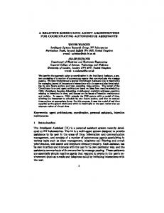
This instance has K = 2 call types and I = 2 agent types, with S1 = {1} and S2 = {1, 2}. Agent costs are computed by setting the parameter ς equals to 0.2 in formula 4. Arrival rates for the two call types are plotted in Figure 1. All SL constraints are enforced in this instance. Four different CPU time budgets were considered: 3, 15, 30 and 60 minutes.. Results, based on r = 32 replications, are displayed in Table 2. 160

140

arrival rates

120

100 type 1 type 2 80

60

40

20 0

2

4

6

8

10

12

14

16

18

20

22

24

26

28

30

32

34

36

periods

Figure 1: Small center: arrival rates

Several observations can be made from Table 2. First, CP-IP is almost always able to find feasible solutions to the problem and most of them are very good. In fact, the only case where solutions are more expensive than those obtained with TS, and these are infeasible, is when n = 120. This seems to indicate that this might be too small a value for n. On the other hand, the results obtained for the three 15

Case Algorithm 1 2 3 4

CP-IP TS CP-IP TS CP-IP TS CP-IP TS

n

CPUavg sec. 50 136 162 800 914 898 1000 1774 1753 1000 3694 3453 n2

120 120 1500 1500 1600 2800 2000 6000

Med P1∗ cost 36.91 0 35.60 0 35.17 100 35.59 0 35.17 75 35.67 0 35.17 100 35.67 0

Min cost 36.31 35.60 35.13 35.59 35.03 35.67 35.03 35.67

P∗

Gperiod

Gcall,period

100 0 100 0 87 0 100 0

0 0.81 0 0.94 0 0.79 0 0.79

0 0 0 0 0.15 0 0 0

Table 2: Small center: results obtained with CP-IP and TS for different CPU time budgets

larger values of n are quite similar and setting n to 1500 is probably sufficient for this small center. It is also interesting, and rather surprising, to find out that all runs of TS failed to find a feasible solution, even though constraint violations were always inferior to 1%. The solutions produced by TS are also more expensive than the ones obtained with CP for large enough n. Such an outcome in not surprising considering the inherent shortcomings of the method. A closer examination of the distribution of the cost of solutions reveals that, except for CP-IP with n = 120, these costs vary very little. With TS, all runs with the same computing budget return in fact the same cost value. In practice, a manager might be willing to use almost-feasible solutions, considering the fact that the center will always experience stochastic variation in the arrival process and the SL in any case. For this reason, it is probably useful to report slightly infeasible solutions in general, and not only the feasible ones. The best scheduling solutions obtained by CP and TS are described in Table 3. In this table, shift types correspond to the length of the shifts as indicated in Table 1. Both methods return solutions with the same number of agents (31), most of which are specialists (type 1). Further analysis of these solutions reveals that they differ only slightly in terms of the duration of the shifts scheduled, but CP uses more specialists than TS (24 vs 21) and thus gives a cheaper solution. Algorithm Agent type CP-IP TS

1 6 3 6 4

1 2 1 2

2 3 0 1 1

Shift type 3 4 5 3 1 1 0 1 1 3 1 2 0 1 0

6 8 2 7 3

7 2 0 1 1

Table 3: Small center: scheduling solutions

Service levels for the best solution obtained are plotted in Figure 2. We see (1) a wide variation of the SL throughout the day and (2) that calls of type 1 have much better SL than those of type 2. This 16

1

0.9

Service Level

0.8

0.7

0.6

0.5

0.4 1

6

11

16

21

26

31

36

period call type 1

call type 2

aggregate

target for the service levels aggregated by call types

target for the other service levels

Figure 2: Small center: service levels by period imbalance can be explained by the fact that the type 1 calls can be answered by less expensive specialists, while type 2 calls must be handled by generalists. This observation highlights the fact that to ensure a fair treatment of all call types in a real-life setting, it is often necessary to include call-type specific SL constraints (either over the whole day or for each period) in the problem formulation.

4.2

A medium-sized call center

In the medium-sized instances, there are K = 5 call types and I = 15 agent types. Skill sets are displayed in Table 4. The parameter ς used to compute agent costs in formula 4 is now equal to 0.1. Arrival rates for all call types are plotted in Figure 3. Skill Agent types 1 1, 6, 9, 10, 11, 14, 15 2 2, 7, 9, 10, 12, 13, 14, 15 3 3, 8, 13, 15 4 4, 11, 12, 13, 14, 15 5 5, 6, 7, 8, 10, 11, 12, 14, 15 Table 4: Medium-sized center: skill sets

As we already mentioned, we consider two variants of the medium-sized centre: in the first, called M1 , only global and per-period SL constraints are enforced, while the second variant, M2 , also includes disaggregate SL constraints.

Since in practice one may find it hard to satisfy all SL 17

23

arrival rates

18

type 1 type 2 and 4 type 3 and 5

13

8

3 0

2

4

6

8

10

12

14

16

18

20

22

24

26

28

30

32

34

36

periods

Figure 3: Medium-sized center: arrival rates constraints and since real-life call center managers are often more interested by global SL, it seemed interesting to compare these two variants. For each of them, we performed r = 8 replications for several CPU time budgets of 15, 30 and 60 minutes. Because of the larger size of these instances, it was not possible to run CP-IP, since this would have led to unacceptable running times; we used CP-LP instead. The results for M1 and M2 are summarized in Tables 5 and 8. From these tables, one can conclude that most replications of CP-LP return low-cost feasible solutions for both variants, but the cost variation between solutions is more pronounced than for the small center. The quality of solutions also increases significantly with n, which emphasizes the importance of performing long enough simulations in the obtention of good results. Contrary to what was observed for the small center, TS always finds feasible solutions, but their cost is much higher than the cost of CP solutions; in fact, the optimality gap with respect to the best solution found is over 25% for M1 and close to that value for M2 . This shows that large suboptimality gaps with TS do occur in realistic call center settings, and not only in artificial examples. If one compares the best scheduling solutions obtained for M1 with CP and TS (see Tables 6 and 7), one observes that CP not only uses significantly less agents (14 vs 17), but also that these agents have on average a smaller number of skills (2.50 vs 2.76) and work shorter hours (more than 10 minutes less a day, on average) . Similar results are observed for M2 in Tables 9 and 10. When we compare the value of the best solutions obtained by CP for M1 and M2 , we notice that the solution obtained for M1 is cheaper, which is exactly what was to be expected since M1 turns out to be a relaxation of M2 . In fact, the most interesting conclusion that one could draw here is that the increase in cost incurred when imposing the disaggregate SL constraints is rather marginal. We have 18

Case Algorithm 1 2 3

n

CP-LP TS CP-LP TS CP-LP TS

300 1200 600 2400 1000 3000

CPUavg sec. 100 855 897 100 1598 1774 400 2686 2793 n2

Min cost 18.33 21.83 17.56 21.72 17.36 21.69

Med P1∗ cost 18.85 0 21.83 0 18.43 0 21.72 0 17.66 25 21.69 0

P∗

Gperiod

87 100 75 100 87 100

0.51 0 0.41 0 0.02 0

Table 5: M1 : results obtained with CP-LP and TS for different CPU time budgets

1 2 agents CP 4 1 agents TS 5 1

shift types 3 4 5 6 1 0 2 4 1 2 1 6

total 7 2 1

14 17

Table 6: M1 : scheduling solutions

plotted the SL curves by period for these solutions in Figure 4. These curves clearly show that the overall SL undergoes significant variations throughout the day; we also note that the two patterns observed are quite different, which highlights the importance of imposing SL constraints by type of calls.

4.3

A larger call center

The larger center instances have K = 20 call types and I = 35 agent types. Skill sets are displayed in Table 11. Agent costs are computed with ς = 0.1. For this larger example, we only consider SL constraints by period, plus the global SL constraint. Two CPU time budgets are examined: 5 and 10 hours. As for the medium-sized center, the CP-LP version of CP is run. All results are obtained by performing r = 8 replications. One of our objectives with this larger example is to show that the performance of CP does not depend on the particular structure of the shifts. We thus consider again two variants: L36 , which uses the 9-hour working day and the same shift structure as the previous examples, and L52 , which has a working day starting at 8:00 AM and ending at 9:00 PM; in that variant, the total number of periods

1 CP 1 TS 0

2 0 0

3 1 3

4 5 1 1 0 0

6 0 1

7 1 2

agent types 8 9 10 11 12 13 2 0 1 1 1 2 2 0 1 1 1 2

14 15 0 2 1 3

Table 7: M1 : total number of agents of each type in the scheduling solutions

19

0.99

Service Level

0.94

0.89

0.84

0.79 1

6

11

16

21

26

period QoS Medium 1

QoS Medium 2

Target

Figure 4: Service level by period for M1 and M2

20

31

36

Case Algorithm 1 2 3

CP-LP TS CP-LP TS CP-LP TS

n

CPUavg sec. 100 828 876 100 1751 1677 100 3520 3212 n2

400 600 400 1500 400 3000

Min cost 18.48 21.58 18.11 21.65 17.92 21.80

Med cost 18.98 21.58 18.97 21.65 18.57 21.80

P1∗

P∗

Gperiod

Gcall,period

0 0 0 0 0 0

87 100 87 100 75 100

0.58 0 0.54 0 0.28 0

0 0 0 0 0 0

Table 8: M2 : results obtained with CP and TS varying the CPU time budget

1 2 agents CP 4 0 agents TS 3 1

shift types 3 4 5 6 1 1 0 6 1 2 1 7

total 7 2 2

14 17

Table 9: M2 : scheduling solutions

is 52 and all the shifts have a fixed length of 7.5 hours, thus yielding a total of 123 different shifts (considering also shifts starting at 1:00 PM and 1:30 PM in order to cover the additional periods). Arrival rates for both variants are plotted in Figure 5 (only the rates of the first 36 periods apply to L36 ). Results obtained for the L36 variant are displayed in Table 12. On this larger problem, CP has difficulty finding a feasible solution with the smaller computing budget. In fact, only two runs out of 8 succeed in finding feasible solutions to the problem, even though constraint violations might not be severe. This situation is clearly alleviated by allotting more CPU time. Furthermore, with more time, CP finds significantly better solutions. TS always finds feasible solutions within the allotted computing budget, but the solutions returned are on average 20% more expensive than those obtained with CP. This confirms our observations of the previous section regarding the poor performance of TS. Surprisingly, increasing the CPU budget does not improve the quality of the results obtained with TS. In fact, with more time, it returns inferior solutions. This is because the method obtains a different staffing solution in the first step; while this solution might track more closely the call arrival curve, it ends up leading to a poorer scheduling solution. A close examination of the relative cost distributions of solutions highlights the fact that, in the case of TS, all replications produce identical, and largely suboptimal, solutions. When one examines the best scheduling solutions obtained by CP and TS (see Table 13), the reason for the lower cost of the CP solution becomes obvious: by resorting to slightly more agents with long shifts, CP is capable of covering the demand with only 52 agents compared to 62 for TS. Results obtained for the L52 variant are reported in Table 14. On this larger problem, a single one of the 8 solutions found by CP-LP, was declared feasible by the 50,000-day simulation, but it is an excellent solution with a cost of 131.7. With more time, CP returned 4 feasible solutions out 21

1 CP 0 TS 0

2 1 0

3 1 2

4 5 0 1 0 0

6 1 2

agent types 7 8 9 10 11 12 13 0 3 1 0 1 1 2 2 3 0 1 1 1 2

14 15 1 1 1 2

Table 10: M2 : total number of agents for each type in the scheduling solutions

26

arrival rates

21

16

11

6

1 0

2

4

6

8

10

12

14

16

18

20

22

24

26

28

30

32

34

36

38

40

42

44

46

periods type 1 and 14 type 4 type 8 and 20 type 17

type 2 type 5 type 9 type 19

type 3 types 6,7,10,11,13,15,16,18 type 12

Figure 5: Larger instances: arrival rates

22

48

50

52

Skill Agent types 1 10, 12, 14, 16, 35 2 1, 3, 5, 7, 9, 17 3 3, 11, 13, 18 4 1, 4, 10, 19, 35 5 2, 6, 7, 9, 20 6 4, 8, 11, 12, 21 7 4, 5, 9, 11, 13, 14, 22 8 1, 3, 4, 5, 9, 23 9 4, 5, 8, 12, 13, 24 10 4, 7, 9, 11, 25, 35 11 3, 8, 10, 13, 14, 26 12 1, 4, 6, 9, 14, 27 13 7, 8, 12, 14, 28 14 1, 5, 6, 13, 29 15 4, 9, 11, 30, 35 16 1, 5, 10, 31 17 2, 3, 12, 13, 32 18 1, 7, 11, 14, 33 19 2, 5, 7, 11, 12, 13, 34 20 2, 4, 6, 8, 15, 35 Table 11: The skill sets for the larger instances

of 8 runs, but these turned out to be inferior to the one found in 5 hours, probably due to simulation noise. Overall, these results emphasizes the importance of performing several trial runs when using this type of approach. All the solutions returned by TS were declared feasible, but they are significantly more expensive, with a cost of 156.1. This is once more an example of the large suboptimality gaps produced by the TS method. Table 15 displays the best solutions found by CP-LP and by TS for the L52 instance. In the table, agent types are regrouped by cost, which is equivalent to grouping them by number of skills, since in this variant, because all agents work 7.5-hour shifts, agent costs depend only upon their skill Case Algorithm 1 2

CP-LP TS CP-LP TS

n 400 1500 500 2400

CPUavg min. 50 288 299 50 577 598 n2

Min cost 82.02 96.08 78.87 102.87

Med cost 82.20 96.08 81.80 102.87

P1∗

P∗

Gperiod

0 0 25 0

25 100 87 100

0.25 0 0.15 0

Table 12: L36 : results obtained with CP-LP and TS for different CPU time budgets

23

shift types 1 2 3 4 5 6 agents CP 17 1 4 7 3 17 agents TS 25 4 4 4 2 17

total 7 3 6

52 62

Table 13: L36 : scheduling solutions Case Algorithm 1 2

CP-LP TS CP-LP TS

n 300 1500 400 1800

CPUavg minutes 50 296 262 50 588 542 n2

Min cost 130.8 156.1 133.5 156.1

Med cost 133.6 156.1 137.7 156.1

P1∗

P∗

Gperiod

12 0 0 0

12 100 50 100

0.54 0 0.44 0

Table 14: L52 : results obtained with CP-LP and TS for different CPU time budgets

sets. The table gives the total number of agents of each group (each cost) in the solution. When we analyze the results, we first remark that CP-LP uses only 96 agents compared to 107 for TS. We also note that several of the agents in the CP solution are specialists, while TS uses a large number of expensive generalists with 7 skills. These two factors combined explain the large difference in cost. agent type cost CP-LP TS 4 1.8 1 1 1,5,9,11,13 1.6 12 32 7,12,14 1.5 29 18 2,3,8,35 1.4 15 33 6,10 1.3 24 23 15,. . . ,34 1.0 15 0 total number 96 107 total cost 131.7 156.1 Table 15: L52 : a summary of the best feasible solutions found by CP-LP and by TS

Our motivation for investigating the 52-period example was to verify that CP performed correctly for instances with a different shift structure. Our results confirm this, but at the same time they highlight one of the potential shortcomings of the approach, which is that, because of simulation noise, one may end up with no feasible solution, even though several near-feasible solutions may have been identified. We address this issue in the next subsection.

4.4

Getting more feasible results

Empirical results show that, as problem instances become larger and more complex, there is a definite possibility that CP would return a set of low-cost, but only nearly-feasible solutions. While this 24

may be acceptable in some practical settings, it is nonetheless annoying to be unable to provide the call center manager with a solution that meets all his/her requirements. A simple and attractive way of tackling this problem consists in slightly increasing the right-hand side value of the SL constraints when applying the algorithm (except obviously for the final long simulation that is used to determine the feasibility of solutions). It should be noted that this idea is not specific to the CP procedure and could therefore be applied with any other solution approach. We first tested this idea on the L52 instance, using values of 0.81 and 0.82 as target SL for all periods. We combined these tests with experiments on the value of the threshold δ that is used for rounding continuous solutions to integer ones in CP-LP. The rationale for investigating different values of δ is that the rounding procedure used in CP-LP introduces a heuristic element in what would otherwise be an exact procedure and that selecting the best value for this threshold is far from obvious. In our experiments, we considered three different values of δ (0.5, 0.6 and 0.7) for CPU budgets of 5 and 10 hours and ran 8 replications in each case. All 48 runs performed for each of the two target values turned out to be feasible for the 50,000-day simulation! Furthermore, one of these runs returned a solution that was significantly better than the best solution found before (cost of 130.5 vs 131.7). The results obtained for a SL target of 0.81 are summarized in Table 16. These results show that the value selected for δ seems to have a slight, but not critical impact on the quality of the solutions obtained. In fact, it seems to be much more important to make sure that the runs that are made do produce feasible solutions, in order to have a larger set to choose from. We then CPU budget hours 0.5 5 10 0.6 5 10 0.7 5 10 δ

Min cost 132.10 132.30 130.50 135.30 132.50 131.60

Med cost 134.85 136.80 133.55 138.60 135.20 138.05

Worst SL ≥ 0.8 ≥ 0.8 ≥ 0.8 ≥ 0.8 ≥ 0.8 ≥ 0.8

Table 16: L52 : results obtained with a target SL of 0.81

ran CP-LP with the original 0.80 target value for different values of δ . These tests clearly showed that modifying δ alone was not sufficient to consistently obtain feasible solutions, since more than half of these runs returned infeasible solutions. However, they did allow us to find an even cheaper feasible solution with a cost 130.4. We also ran the algorithm with a target SL value of 0.81 for the other instances (keeping the value of δ unchanged at 0.5). The results that we otained can be summarized as follows: • For the small center, all runs returned feasible solutions, which was not surprising considering 25

previous results, but these solutions were not better than the ones obtained previously. • For the medium-sized instances, all runs succeeded in producing feasible solutions and improved solutions were obtained both for the M1 and M2 instances (with respective costs of 17.22 and 17.39). • For the L36 instance, 15 of the 16 runs yielded a feasible solution, but never better than the best one found with an SL target of 0.8. Overall, slightly increasing the value of the SL target value is a useful device for making sure that the method will return feasible solutions. However, there is no guarantee that better solutions will be found by doing so. In fact, the variability of the results that we observed in this respect once again highlights the stochastic nature of the proposed approach, which cannot be avoided considering the significant amount of noise in the simulations.

4.5

The impact of flexibility

We performed another series of numerical experiments to quantify empirically the impact of the flexibility provided by a rich set of shift types. Those experiments were performed on the small center of subsection 4.1. We considered three sets of shift types: the original one with all 285 shifts, a slightly reduced one with 267 shifts, obtained by deleting the 26-period and some 36-period shifts, and adding some 35-period ones, and finally a much more restricted set in which we only allow the 105 7.5-hour shifts. The staffing solutions corresponding to the best scheduling solutions obtained for these three cases are plotted in Figure 6, along with the optimal staffing solution computed by considering each period individually. Three main conclusions can be drawn from this figure: 1. As shown by the solution with 285 shifts, if enough flexibility is introduced in the set of available shifts, it is possible to find schedules that track closely the staffing requirements. 2. Even a slight decrease in flexibility (e.g., by going from 285 to 267 shifts) can lead to a significant overstaffing in some periods. 3. Schedules with a relatively small number of fixed-length shifts (the 105-shift case) are bound to suffer from major overstaffing. It follows that, while the complexity of the scheduling problem significantly increases with the number of available shifts, there are definite benefits to be reaped from the introduction of more varied shift types.

26

48

total number of agents

43

38

33

28

23

18

13 0

1

2

3

4

5

6

7

8

9 10 11 12 13 14 15 16 17 18 19 20 21 22 23 24 25 26 27 28 29 30 31 32 33 34 35 36

period Optimal Staffing

Staffing with 105 shifts

Staffing with 267 shifts

Staffing with 285 shifts

Figure 6: Small center: staffing solutions with 105, 267 and 285 shift types

5

Conclusion

We have proposed in this paper a simulation-based methodology to optimize agent scheduling over one day in a multiskill call center. Even though the use of common random numbers reduces the simulation noise (or variance) significantly, there is still a fair amount of randomness in the solution provided by the algorithm, mainly due to the fact that the simulation length must be kept short (because the estimation of each subgradient requires simulations at up to thousands of different parameter values). Yet, to our knowledge, better solutions are found with this approach than with any other method we know. In particular, during the development of the cutting plane algorithm, we also implemented simultaneously a metaheuristic method based on neighborhood search combined with queueing approximation, along the lines of Avramidis et al. (2007a), but we were unable to make it competitive for solving the scheduling problem. In practice, one may run the algorithm a few times (e.g., overnight) to obtain a few solutions and retain the best found. We also showed that by slightly perturbing the SL targets, it is possible to overcome some of the problems caused by the presence of the simulation noise and thus to greatly increase the probability of obtaining feasible, high-quality solutions. Future research on this problem include the search for faster ways of estimating the subgradients (by simulation), refining the algorithm to further reduce the noise in the returned solution, and extending the technique to simultaneously optimize the scheduling and the routing of calls (via dynamic rules).

27

Acknowledgements This research has been supported by Grants OGP-0110050, OGP38816-05, and CRDPJ-320308 from NSERC-Canada, and a grant from Bell Canada via the Bell University Laboratories, to the second and third authors, and a Canada Research Chair to the third author. The fourth author benefited from the support of the University of Calabria and the Department of Electronics, Informatics and Systems (DEIS), and her thanks also go to professors Pasquale Legato and Roberto Musmanno.

References J. Atlason, M. A. Epelman, and S. G. Henderson. Call center staffing with simulation and cutting plane methods. Annals of Operations Research, 127:333–358, 2004. A. N. Avramidis, A. Deslauriers, and P. L’Ecuyer. Modeling daily arrivals to a telephone call center. Management Science, 50(7):896–908, 2004. A. N. Avramidis, W. Chan, and P. L’Ecuyer. Staffing multi-skill call centers via search methods and a performance approximation. IIE Transactions, 2007a. to appear. A. N. Avramidis, M. Gendreau, P. L’Ecuyer, and O. Pisacane. Simulation-based optimization of agent scheduling in multiskill call centers. In Proceedings of the 2007 Industrial Simulation Conference, pages 255–263. Eurosis, 2007b. S. Bhulai, G. Koole, and A. Pot. Simple methods for shift scheduling in multi-skill call centers, 2007. Manuscript, available at http://www.cs.vu.nl/~koole/research. L. Brown, N. Gans, A. Mandelbaum, A. Sakov, H. Shen, S. Zeltyn, and L. Zhao. Statistical analysis of a telephone call center: A queueing-science perspective. Journal of the American Statistical Association, 100:36–50, 2005. E. Buist and P. L’Ecuyer. A Java library for simulating contact centers. In Proceedings of the 2005 Winter Simulation Conference, pages 556–565. IEEE Press, 2005. Bureau of Labor Statistics. Occupational Outlook Handbook, Customer Service Representatives, 2006-07 Edition. 2007. U.S. Department of Labor. Available online at http://www.bls.gov/ oco/ocos280.htm (last accessed February 14, 2007). M. T. Cez¸ik and P. L’Ecuyer. Staffing multiskill call centers via linear programming and simulation. Management Science, 53, 2007. To appear.

28

CRTC. Final standards for quality of service indicators for use in telephone company regulation and other related matters, 2000. Canadian Radio-Television and Telecommunications Commission, Decision CRTC 2000-24. See http://www.crtc.gc.ca/archive/ENG/Decisions/ 2000/DT2000-24.htm. N. Gans, G. Koole, and A. Mandelbaum. Telephone call centers: Tutorial, review, and research prospects. Manufacturing and Service Operations Management, 5:79–141, 2003. L. V. Green, P. J. Colesar, and J. Soares. An improved heuristic for staffing telephone call centers with limited operating hours. Production and Operations Management, 12:46–61, 2003. S. Halfin and W. Whitt. Heavy-traffic limits for queues with many exponential servers. Operations Research, 29:567–588, 1981. S. Henderson and A. Mason. Rostering by iterating integer programming and simulation. In Proceedings of the 1998 Winter Simulation Conference, volume 1, pages 677–683, 1998. A. Ingolfsson, E. Cabral, and X. Wu. Combining integer programming and the randomization method to schedule employees. Technical report, School of Business, University of Alberta, Edmonton, Alberta, Canada, 2003. Preprint. O. B. Jennings, A. Mandelbaum, W. A. Massey, and W. Whitt. Server staffing to meet time-varying demand. Management Science, 42(10):1383–1394, 1996. E. G. Keith. Operator scheduling. AIIE Transactions, 11(1):37–41, 1979. G. Koole and A. Mandelbaum. Queueing models of call centers: An introduction. Annals of Operations Research, 113:41–59, 2002. A. M. Law and W. D. Kelton. Simulation Modeling and Analysis. McGraw-Hill, New York, NY, third edition, 2000. P. L’Ecuyer. SSJ: A Java Library for Stochastic Simulation, 2004. Software user’s guide, Available at http://www.iro.umontreal.ca/~lecuyer. P. L’Ecuyer, R. Simard, E. J. Chen, and W. D. Kelton. An object-oriented random-number package with many long streams and substreams. Operations Research, 50(6):1073–1075, 2002. V. Mehrotra. Ringing up big business. ORMS Today, 24(4):18–24, October 1997. A. Pot, S. Bhulai, and G. Koole. A simple staffing method for multi-skill call centers, 2007. Manuscript, available at http://www.cs.vu.nl/~koole/research.

29

R. Stolletz and S. Helber. Performance analysis of an inbound call center with skill-based routing. OR Spectrum, 26:331–352, 2004. G. M. Thompson. Labor staffing and scheduling models for controlling service levels. Naval Research Logistics, 8:719–740, 1997. S. Vogel. A stochastic approach to stability in stochastic programming. Journal of Computational and Applied Mathematics, 56:65–96, 1994.

30