Optimizing Grid Site Manager Performance with Virtual Machines Ludmila Cherkasova, Diwaker Gupta
Eygene Ryabinkin, Roman Kurakin, Vladimir Dobretsov
{lucy.cherkasova,diwaker.gupta}@hp.com
{Eygene.Ryabinkin,Roman.Kurakin,Vladimir.Dobretsov}@grid.kiae.ru
Hewlett-Packard Labs Palo Alto, CA 94304, USA
Russian Research Center “Kurchatov Institute” Moscow, Russia
Amin Vahdat
University of California San Diego, CA 92122, USA
[email protected]
Abstract— Virtualization can enhance the functionality and ease the management of current and future Grids by enabling ondemand creation of services and virtual clusters with customized environments, QoS provisioning and policy-based resource allocation. In this work, we consider the use of virtual machines (VMs) in a data-center environment, where a significant portion of resources from a shared pool are dedicated to Grid job processing. The goal is to improve efficiency while supporting a variety of different workloads. We analyze workload data for the past year from a Tier-2 Resource Center at the RRC Kurchatov Institute (Moscow, Russia). Our analysis reveals that a large fraction of Grid jobs have low CPU utilization, which suggests that using virtual machines to isolate execution of different Grid jobs on the shared hardware might be beneficial for optimizing the data-center resource usage. Our simulation results show that with only half the original infrastructure employing VMs (50 nodes and four VMs per node) we can support 99% of the load processed by the original system (100 nodes). Finally, we describe a prototype implementation of a virtual machine management system for Grid computing.
I. I NTRODUCTION One of the largest Grid efforts unfolds around the Large Hadron Collier (LHC) project [1] at CERN. When it begins operations in 2007, it will produce nearly 15 Petabytes (15 million Gigabytes) of data annually. This data will be accessed and analyzed by thousands of scientists around the world. The main goal of the LHC Computing Grid (LCG) is to develop and deploy the computing environment for use by the entire scientific community. The data from the LHC experiments will be distributed for processing, according to a three-tier model as shown in Figure 1. After initial processing at CERN — the Tier-0 center of LCG — this data will be distributed to a series of Tier-1 facilities: large computer centers with sufficient storage capacity for a significant fraction of the data and 24/7 support for the Grid. The Tier-1 centers will, in turn, make data available to Tier-2 centers, each consisting of one or more collaborating computing facilities, which can store sufficient data and provide adequate computing power for specific analysis tasks. Individual scientists will access these facilities through Tier-3 computing resources, which can consist of local clusters in a University Department or even individual PCs, and which may be allocated to LCG on a regular basis. The analysis of the data, including comparison with theoretical simulations, requires of the order of 100,000 CPUs. Thus the strategy is to integrate thousands of computers and dozens of participating institutes worldwide into a global computing resource.
Fig. 1: LHC Vision: Data Grid Hierarchy. The LCG project aims to collaborate and interoperate with other major Grid development projects and production environments around the world. More than 90 partners from Europe, the US and Russia are leading a worldwide effort to re-engineer existing Grid middleware to ensure that it is robust enough for production environments like LCG. One of the major challenges in this space is to build robust, flexible, and efficient infrastructures for the Grid. Virtualization is a promising technology that has attracted much interest and attention, particularly in the Grid community [2], [3], [4]. Virtualization can add many desirable features to the functionality of current and future Grids: • on-demand creation of services and virtual clusters with pre-determined characteristics [5], [6], • policy-based resource allocation and and management flexibility [5], • QoS support for Grid jobs processing [7], • execution environment isolation, • improved resource utilization due to statistical multiplexing of different Grid jobs demands on the shared hardware. Previous work on using virtual machines (VMs) in Grids has focused on the utility of VMs for better customization and administration of the execution environments. This paper focuses on the performance/fault isolation and flexible resource allocation enabled by the use of VMs. VMs enable diverse applications to run in isolated environments on a shared hardware platform and dynamically control resource allocation for different Grid jobs. To the best of our knowledge, this is the first paper to analyze real workload data from a Grid and give empirical evidence for the feasibility of this idea. We show that there is actually a significant economic and
Wall CPU Time and Actual CPU Time per Job (Logscale)
Overall CPU Usage (Wall Time) by Jobs of Different Duration
1
Memory and Virtual Memory Usage
1
1
0.9 0.8
0.8
0.7
0.7
0.5
0.6
0.4
CDF
0.6 CDF
CDF
0.6
0.4
0.5 0.4
0.3
0.3
0.2
0.2
0.2
Job Duration Actual Used CPU Time
0.1 0 0.01
Virtual Memory Physical Memory
0.9
0.8
0.1 Overall_CPU_Usage 0
0.1
1
10
100
1000
10000
Logscale: Duration (min)
(a)
0 0
1000
2000
3000
4000
5000
6000
7000
Duration (min)
(b)
Fig. 2: Basic Trace Characterization.
performance incentive to move to a VM based architecture. We analyze workloads from a Tier-2 Resource Center (a part of the LCG infrastructure) supported by the Russian Research Center “Kurchatov Institute” (Moscow, Russia). Our analysis shows that the machines in the data center are relatively underutilized: 50% of the jobs use less than 2% CPU-time and 70% use less than 14% of cpu-time during their lifetime. However, existing LCG specifications do not support or require time sharing; only a single job runs on a processor at a time. While this simple resource allocation model provides guaranteed access to the requested resources and supports performance isolation between different Grid jobs, it may lead to significant under-utilization of resources. Our results indicate that assigning multiple Grid jobs to the same node for processing may be beneficial for optimized resource usage in the data center. Our analysis of memory usage reveals that for 98% of the jobs virtual memory usage is less than 512 MB. This means that we can spawn 4-8 virtual machines per compute node (with 4 GB of memory) and have no memory contention due to virtualization layer. These statistics provide strong motivation for executing Grid jobs inside different virtual machines for optimized resource usage in data-center. For instance, our simulation results show that a half-size infrastructure augmented with four VMs per node can process 99% of the load executed by the original system (see Section IV). In addition, the introduction of VMs for Grid job execution enables policy-based resource allocation and management in the data center: the administrator can dynamically change the number of physical nodes allocated for Grid jobs versus enterprise applications without degrading performance support for Grid processing. Live migration of VMs makes the management process even more flexible. We next present our analysis of the Grid workload. II. W ORKLOAD A NALYSIS The RRC Kurchatov Institute (RRC-KI) in Moscow contributes a part of their data-center to the LCG infrastructure (100 nodes with Xeon 2.8 GHz CPU processor, 2GB of memory, and 80 GB ATA or SCSI disks). LCG requires access logs for each job to generate the accounting records [8]. We analyzed the access logs for Grid job processing at RRCKI between 04/29/2005 and 05/25/2006, spanning almost 390 days of operation. The original trace has 65,368 entries. Each trace entry has information about the origin of the job, its start and end time, as well as a summary of resources used by the job. For our analysis, we concentrated on the following fields: • start and end times;
0
500
1000
1500
2000
2500
3000
MBytes
(c)
Virtual Organization (VO) that originated the job; CPU time used per job processing (sec)’ • memory and virtual memory used (MB) For CPU time, we make the distinction between Wall CPU Time (WCT) and Actual CPU Time (ACT). WCT is the overall time taken for a job to finish. ACT reflects the actual CPU time consumed by the job. First, we filter the data to remove erroneous entries. There were numerous for failed Grid jobs (jobs that could not be executed or failed due to some mis-configuration): entries with zero job duration (i.e., when start time = end time), as well as entries with zero ACT, or zero memory/virtual memory consumption. After the filtering, 44,183 entries out of the original 65,368 entries are left for analysis. Figure 2(a) shows the Cumulative Distribution Function (CDF) of the job duration: the WCT is shown by the solid line. We can see that there is a large variation in the job durations: • 58% of jobs have a duration less than 10 min; • 91% of jobs have a duration less than 60 min (i.e., 34% of jobs have duration between 10 min and 1 hour); • 96% of jobs have a duration less than 1440 min (i.e., 5% of jobs have duration between 1 hour and 1 day); • 99.96% of jobs have a duration less than 4325 min (i.e., 3.96% of jobs have duration between 1 day and 3 days); The dotted (green) line in Figure 2(a) shows the CDF of the ACT for the jobs. It is evident from the figure that the ACT for a job is typically much lower than the WCT. For example, 95% of the jobs use less than 1 hour of actual CPU time during their processing. Figure 2(b) presents the fraction of wall CPU time summed over jobs of different duration out of the overall CPU time consumed by all the jobs. We can see that longer jobs are responsible for most of the CPU time consumed by the jobs in the entire trace. For example, • jobs that are less than 1 day in duration are responsible for only 20% of all consumed CPU resources while they constitute 91% of all the jobs; • jobs that execute for about 3 days are responsible for 42% of all consumed CPU resources while they constitute only 2% of all the jobs. Finally, Figure 2(c) shows the CDF of memory and virtual memory consumed per job in mega-bytes (MB). For 98% of the jobs virtual memory usage is less than 512 MB. Only 0.7% of the jobs are using more than 1 GB of virtual memory. Such reasonable memory consumption means that we can use 4-8 virtual machines per node with 4 GB of memory and practically support the same memory performance per job. •
•
Fraction of Jobs per User
Fraction of Used Wall Time per User
0.45
0.3 0.25 0.2 0.15 0.1 0.05
CPU-Usage-Efficiency 80
0.45
CPU-Usage-Efficiency (%)
Fraction of Used Wall Time
Fraction of Jobs
90 Wall Time
0.5
0.4 0.35
0 lhcb
CPU-Usage-Efficiency (CPU Usage/Wall time) per User
0.55 Jobs
0.4 0.35 0.3 0.25 0.2 0.15 0.1
fusion
dteam
alice
atlas
cms
fusion
dteam
User
alice
atlas
cms
User
(a)
60 50 40 30 20 10
0.05 0 lhcb
70
(b)
Fig. 4: General per Virtual Organization Statistics.
0 lhcb
fusion
dteam
alice
atlas
cms
User
(c)
CPU-Usage-Efficiency per Job 1 0.9 0.8 0.7 CDF
0.6 0.5 0.4 0.3 0.2 0.1 CPU-Usage-Efficiency 0 0
10
20
30 40 50 60 70 CPU-Usage-Efficiency (%)
80
90
100
Fig. 3: CDF of CPU-Usage-Efficiency per Job. To get a better understanding of CPU utilization, we introduce a new metric called the CPU Usage Efficiency (CUE), defined by the percentage of actual CPU time consumed by a job out of the wall CPU time. That is, CU E = ACT /W CT . Figure 3 shows the CDF of CPU-usage-efficiency per job. For example, • 50% of the jobs use less than 2% of their WCT • 70% of the jobs use less than 14% of their WCT This data shows that CPU utilization is low for a significant fraction of the Grid jobs, and therefore for nodes hosting these Grid jobs. One possible explanation for the low CPU utilization could be a situation where the bandwidth at the Kurchatov Data Center becomes the bottleneck. To verify this, we analyzed the network bandwidth consumption at the gateway to the Kurchatov Data Center for last year, and the analysis showed that the peak bandwidth usage never exceeded 60% of the available bandwidth. This point is important: since there was enough surplus available bandwidth, the low CPU utilization is not because of a network bottleneck within Kurchatov. We suspect that a bottleneck in the upstream network path might be involved, or there might be overhead/inefficiency in the middleware layer. Next, we analyze the origin of Grid jobs: which Virtual Organization (VO) for which jobs? Six major VOs had submitted their jobs for processing. Figure 4(a) shows the percentage of jobs submitted for processing by these different VOs. • LHCb (45% of all the jobs) • FUSION(22.5% of all the jobs) • DTEAM (18% of all the jobs) • ALICE (8% of all the jobs) • ATLAS (4% of all the jobs) • CMS (2.5% of all the jobs) Discovering new fundamental particles and analyzing their properties with the LHC accelerator is possible only through statistical analysis of the massive amounts of data gathered
by the LHC detectors ATLAS, CMS, ALICE and LHCb, and detailed comparison with compute-intensive theoretical simulations. So these four VOs are directly related to LHC project. DTEAM is the VO for the Grid users in Central Europe and infrastructure testing. FUSION is a VO for researchers in plasma physics and nuclear fusion. Figure 4(b) shows percentage of wall CPU time consumed by different VOs over duration of the entire trace. Grid jobs from LHCb significantly dominate resource usage in Kurchatov data-center: they consumed 50% of overall used CPU resources. Finally, Figure 4(c) presents CPU-usage-efficiency across different VOs. Here, we can see that Grid jobs from CMS [9] and ATLAS [10] have significantly higher CPU utilization during their processing (85% and 70% relatively) compared to the remaining VOs. Understanding workload characteristics of different VOs is very useful for design of efficient VMs/jobs placement algorithm. While the analyzed workload is representative and covers 1-year of Grid job processing in Kurchatov Data Center, we note that our analysis provides only a snapshot of overall Grid activities: Grid middleware is constantly evolving, as is the Grid workload itself. However, the current Grid infrastructure inherently faces potential inefficiencies in resource utilization due to the myriads of middleware layers and the complexity introduced by distributed data storage and execution systems. The opportunity for improvement (using VMs) will depend on the existing mixture of Grid jobs and their types: what fraction of the jobs represent computations that are remote data dependent (e.g., remote data processing) and what fraction of the jobs are pure CPU intensive (e.g., a simulation experiment). III. G RID J OB R ESOURCE U SAGE P ROFILING To better understand the resource usage during Grid job processing, we implemented a monitoring infrastructure and collected a set of system metrics for the compute nodes in RRC-KI, averaged over 10 sec intervals for one week in June, 2006. Since I/O operations typically lead to lower CPU utilization, the goal was to build Grid job profiles (metric values as a function of time) to reflect I/O usage patterns, and analyze whether local disk I/O or networking traffic may be a cause of the low CPU utilization per job. During this time 1372 Grid jobs were processed and 90% of the processed jobs had CPU-usage-efficiency less than 10%. For each Grid job, we consider the following metrics: • The percentage of CPU time that is spent in waiting for disk I/O events;
Jobs Profile over Time: Blocked CPU Time on Disk I/O Events
Jobs Profile over Time: Incoming Network Traffic
Jobs Profile over Time: Outgoing Network Traffic
1
1
1
0.95
0.9
0.9
0.8
0.8
0.7
0.7
0.9
0.8 0.75 0.7
CDF of Jobs
CDF of Jobs
CDF of Jobs
0.85
0.6 0.5
0.6 0.5
0.65 0.4 0.6
99th 90th 80th
0.55
0.4 99th 90th 80th
0.3
0.5
0.2 0
10
20 30 40 50 60 CPU Time Waiting for Disk I/O Events (%)
(a)
70
0.2 0.1
1
10 100 KB/sec (Logscale)
(b)
•
1000
10000
Fig. 5: Grid Job I/O usage Profiles.
Incoming network traffic in KB/sec; Outgoing network traffic in KB/sec; To simplify the job profile analysis, we present the profiles as CDFs for each of the three metrics. This way, we can see what percentage of CPU time is spent while waiting for disk I/O events during each 10 sec time interval over a job’s lifetime. For understanding the general trends, we plot 80-th, 90-th, and 99-th percentile for each metric in the job profile. For example, to construct the CDF corresponding to the 80-th percentile, we would look at the metric profile for each job and collect the 80-th percentile points, and then plot the CDF of these collected points. Figure 5(a) plots the Grid job profiles related to local disk I/O events. It shows that • for 80% of the time nearly 90% of the jobs have no CPU time waiting on disk events, and for remaining 10% of jobs CPU waiting time does not exceed 5%; • for 90% of the time approximately 80% of the jobs have no CPU time waiting on disk events, and for remaining 20% of jobs CPU waiting time does not exceed 10%; • for 99% of the time nearly 50% of the jobs have no CPU time waiting on disk events, for remaining 45% of jobs CPU waiting time in this 1% of time intervals does not exceed 10%, and only 5% of the jobs have CPU time waiting in the range 10-60%. Hence, we can conclude that local disk I/O can not be a cause of low CPU utilization. Figures 5(b) and 5(c) summarize the incoming/outgoing network traffic profiles across all jobs (note the graphs use logscale for X-axes). One interesting (but expected observation) is that there is a higher volume of incoming networking traffic compared to the volume of outgoing networking traffic. The networking infrastructure in the Kurchatov Data Center is not a limiting factor: the highest volume of incoming networking traffic is in the range of 1 MB/sec to 10MB/sec and is observed only for 1% of time intervals and 10% of Grid jobs. More typical behavior is that 70%-80% of the jobs have a consistent (relatively small) amount of incoming/outgoing network traffic in 1% of time intervals. Additionally, 40% of grid jobs have incoming/outgoing network traffic in 10% of time intervals, while only 10%-20% of jobs have incoming/outgoing network traffic in 20% of time intervals. While it does not explain completely why CPU utilization is low for large fraction of the Grid jobs, our speculation is that it might be caused due to inefficiencies in remote data transfers and by slowdown in related data processing. •
99th 90th 80th
0.3 0.1
1
10 KB/sec (Logscale)
100
1000
(c)
IV. S IMULATION R ESULTS To analyze potential performance benefits of introducing VMs, we use a simulation model with the following features and parameters: • N umN odes - the number of compute nodes that can be used for Grid job processing. By setting this parameter to unlimited value, we can find the required number of nodes under different scenarios (combination of the other parameters in the model). When N umN odes is set to a number less than the minimum nodes required under a certain scenario, the model implements admission control, and at the end of the simulation the simulator reports the number (percentage) of rejected jobs from a given trace. • N umV M s - the number of VMs that can be spawned per node. N umV M s = 1 corresponds to the traditional Grid processing paradigm with no virtual machines and one job per node. When setting N umV M s = 4 no more than four VMs are allowed to be created per node. • Overbooking - the degree of over booking (or under booking) of nodes when assigning multiple VMs (jobs) per node. Overbooking = 1 corresponds to the ideal case where the virtualization layer does not introduce additional performance overhead. Using Overbooking ≤ 1, we can evaluate performance benefits solution under different virtualization overheads. By allowing Overbooking ≥ 1, we can evaluate the effect of limited time overbooking of the node resources. This may lead to potential slowdown of Grid job processing: processing time slowdown is another valuable metric for evaluation. Note that we don’t experiment with Overbooking > 1 in this work. The model implements a least-loaded placement algorithm: an incoming job is assigned to the least-loaded node that has a spare VM that can be allocated for job processing. This model provides optimistic results compared to the real case scenario because the placement algorithm above has “perfect” knowledge about required CPU resources of each incoming job and therefore its performance is close to the optimal. First, we used this model to simulate the original Grid job processing in Kurchatov Data Center over time (N umN odes = unlimited, N umV M s = 1, Overbooking = 1). Figure 6(a) shows the number of concurrent Grid jobs over time, i.e., the number of CPUs allocated and used over time. Figure 6(b) shows the actual utilization of these nodes, i.e, the combined CPU requirements of jobs
100 AllocatedCPUs NumCPUs
80 60 40 20 0 0
50
100
150
200 Time (days)
250
300
350
400
(a) 100 Combined_ActuallyUsedCPUs NumCPUs
80 60 40 20 0 0
50
100
150
200 Time (days)
250
300
350
400
(b)
Fig. 6: Original Grid Job Processing in Kurchatov Resource Center Over Time. in progress, based on their actual CPU usage. The X-axes is in days since the beginning of the trace. While RRCKI advertised 100 compute nodes available for processing throughput last year, there are rare days when all of these nodes are actually used. Figure 6(b) shows that the allocated CPUs are significantly underutilized most of the time. We simulated processing of the same job trace under different scenarios with limited available CPU resources: • N umN odes = 40, 50, 60; • N umV M s = 1, 2, 4, 6, 8; • Overbooking = 0.8, 0.9, 1.0. Table I shows the results: the percentage of rejected jobs from the overall trace under different scenarios. The simulation results for different values of Overbooking = 0.8, 0.9, 1.0 are the same, this is why we show only one set of the results. It means that even with virtualization overhead of 20% the consolidation of different grid jobs for processing on a shared infrastructure with VMs is highly beneficial and there is enough spare capacity in the system to seamlessly absorb an additional virtualization overhead. 40 nodes 50 nodes 60 nodes
Orig 20.1% 10.9% 4.73%
2 VMs 4.72% 1.51% 0.53%
4 VMs 2.75% 1.08% 0.49 %
6 VMs 2.52% 1.06% 0.48%
8 VMs 2.51% 1.05% 0.48%
number of VMs per node to six or eight provides almost no additional reduction in number of rejected jobs. This indicates the presence of diminishing returns: arbitrarily increasing the multiplexing factor will not improve performance. Thus with a half-size infrastructure and use of VMs (50 nodes and four VMs per node) we can process 99% of the load processed by the original system with 100 nodes. V. P ROTOTYPE We now describe our prototype design built on top of the Xen VMM. Let us briefly look at the current work-flow for executing a Grid job at Kurchatov shown in Figure 7:
Fig. 7: Original work-flow for a Grid job. •
TABLE I: Percentage of rejected Grid jobs during processing on limited CPU resources with VMs. First of all, we evaluated the scenario when the original system has a decreased number of nodes. As Table I shows, when the original system has 40 nodes the percentage of rejected jobs reaches high 20%, while under scenario when these 40 nodes support 4 VMs per node the rejection rates are only 2.75% for the overall trace. Another observation is that increasing the number of VMs per node from two to four has a significant impact on decreasing the number of rejected jobs. Further increasing the
•
•
A Resource Broker (RB) is responsible for managing Grid jobs across multiple sites. The RBs sends jobs to Computing Elements (CE). CEs are just Grid gateways to computing resources (such as a Data Center). CEs run a batch system (in particular, LCG uses Torque with the MAUI job scheduler [11]). The job scheduler determines the machine — called a Worker Node (WN) — that should host the job. a local job execution service is notified of a new job request. A job execution script (Grid task wrapper) is passed to the job execution service and the job is executed on the WN. The job script is responsible for retrieving in the necessary data files for the job, exporting the logs
to the RB, executing the job and doing cleanup upon job completion. The goal is to modify the current work-flow to use VMs. At a high level, the entry point for VMs in the system are the worker nodes; we want to immerse each WN within a VM. The interaction with the job scheduler also needs to be modified. In the existing model, the scheduler picks a WN using some logic, perhaps incorporating resource utilization. When VMs are introduced, the scheduler needs to be made VM aware. Our prototype is built using Usher [12] – a virtual machine management suite. We extended Usher to expose additional API required for our prototype as shown in Figure 8. The basic architecture of Usher is as follows: • Each physical machine provisioned in the system runs a Local Node Manager (LNM). The LNM is responsible for managing VMs on that physical machine. It exposes API to create, destroy, migrate and configure VMs. Additionally, it also monitors the resource usage for the machine as a whole as well as for each VM individually and exposes API for resource queries. • A central controller is responsible for co-ordinating the management tasks across the LNMs. Clients talk to the controller and the controller is responsible for dispatching the request to the appropriate LNM.
(just like it currently queries Torque for state of physical machines and processes) and make better informed decisions about VM creation and placement. Our system has been deployed on a test-bed at RRCKI and work is underway to evaluate different policies for Grid job scheduling. We hope to gradually increase the size of the test-bed and plug it into the production Grid workflow, to enable statistical comparison with the original setup. Virtual machine migration is also critical to efficiently utilizing resources. Migration brings in many more policy decisions such as: which VM to migrate? when to migrate? where to migrate? how many VMs to migrate? Some earlier work on dynamic load balancing [13] showed that performance benefits of policies that exploit pre-emptive process migration are significantly higher than those of non pre-emptive migration. We expect to see similar advantages for policies that exploit live migration of VMs. VI. C ONCLUSION Over the past few years, the idea of using virtual machines in a Grid setting has been suggested several times. However, most previous work has advocated this solution from a qualitative, management-oriented viewpoint. In this paper, we make the first attempt to establish the utility of using VMs for Grids from a performance perspective. Using real workload data from a Tier-2 Grid site, we give empirical evidence for the feasibility of VMs and using simulations we quantify the benefits that VMs would give over the classical Grid architecture. We also describe a prototype implementation for such a deployment using the Xen VMM. R EFERENCES
Fig. 8: VM Management System Architecture. The modular architecture and API exposed by Usher made it very easy to implement a “policy daemon” geared towards our use case. We are, in fact, experimenting with several policy daemons varying in sophistication to evaluate the trade-off between performance and overhead. An example of a simple policy would be to automatically create VMs on machines that are not being utilized “enough”, where the definition of “enough” is governed by several parameters such as the CPU load, available memory, number of VMs already running on a physical machine etc. The policy daemon periodically looks at the resource utilization on all the physical machines and spawns new VMs on machines whose utilization is low. Each new VM basically boots as a fresh Worker Node. When the VM is ready, it notifies Torque (the resource manager) that it is now available and then Maui (the scheduler) can schedule jobs on this new VM as if it were any other compute node. When a job is scheduled on the VM, a prologue script makes sure that the VM is re-claimed once the job is over. This approach is attractive because it requires no modifications to Torque and Maui. This policy daemon, albeit simple, can be inefficient if there are not enough jobs in the system – it would pre-emptively create VMs which would then go unused. A more sophisticated policy daemon requires extending Maui: using the Usher API, Maui can itself query the state of physical machines and VMs
[1] “LCG project.” http://lcg.web.cern.ch/LCG/. [2] I. Krsul, A. Ganguly, J. Zhang, J. A. B. Fortes, and R. J. Figueiredo, “VMPlants: Providing and Managing Virtual Machine Execution Environments for Grid Computing,” in SC ’04: Proceedings of the 2004 ACM/IEEE conference on Supercomputing, (Washington, DC, USA), p. 7, IEEE Computer Society, 2004. [3] S. Adabala, V. Chadha, P. Chawla, R. Figueiredo, J. Fortes, I. Krsul, A. Matsunaga, M. Tsugawa, J. Zhang, M. Zhao, L. Zhu, and X. Zhu, “From virtualized resources to virtual computing grids: the In-VIGO system,” Future Gener. Comput. Syst., vol. 21, no. 6, pp. 896–909, 2005. [4] K. Keahey, K. Doering, and I. Foster, “From Sandbox to Playground: Dynamic Virtual Environments in the Grid,” in Proceedings of the 5th International Workshop in Grid Computing, 2004. [5] J. S. Chase, D. E. Irwin, L. E. Grit, J. D. Moore, and S. E. Sprenkle, “Dynamic Virtual Clusters in a Grid Site Manager,” in HPDC ’03: Proceedings of the 12th IEEE International Symposium on High Performance Distributed Computing (HPDC’03), (Washington, DC, USA), p. 90, IEEE Computer Society, 2003. [6] R. J. Figueiredo, P. A. Dinda, and J. A. B. Fortes, “A Case For Grid Computing On Virtual Machines,” in ICDCS ’03: Proceedings of the 23rd International Conference on Distributed Computing Systems, (Washington, DC, USA), p. 550, IEEE Computer Society, 2003. [7] K. Keahey, I. Foster, T. Freeman, and X. Zhang, “Virtual Workspaces: Achieveing Quality of Service and Quality of Life in the Grid,” in Scientific Programming Journal, 2006. [8] “LCG accounting proposal.” http://goc.grid-support.ac. uk/gridsite/accounting/apel-schema.pdf. [9] “CMS.” http://cms-project-ccs.web.cern.ch/. [10] “ATLAS.” http://atlas.web.cern.ch/. [11] “Cluster, grid and utility computing products.” http://www. clusterresources.com/pages/products.php. [12] T. U. Team, “Usher: A Virtual Machine Scheduling System.” http: //usher.ucsdsys.net/. [13] M. Harchol-Balter and A. Downey, “Exploiting Process Lifetime Distributions for Dynamic Load Balancing,” in Proceedings of ACM Sigmetrics ’96 Conference on Measurement and Modeling of Computer Systems, (SIGMETRICS 96), 1996.