1 SEPTEMBER 2005
SEVERIJNS AND HAZELEGER
3527
Optimizing Parameters in an Atmospheric General Circulation Model C. A. SEVERIJNS
AND
W. HAZELEGER
Royal Netherlands Meteorological Institute, De Bilt, Netherlands (Manuscript received 2 August 2004, in final form 9 December 2004) ABSTRACT An efficient method to optimize the parameter values of the subgrid parameterizations of an atmospheric general circulation model is described. The method is based on the downhill simplex minimization of a cost function computed from the difference between simulated and observed fields. It is used to find optimal values of the radiation and cloud-related parameters. The model error is reduced significantly within a limited number of iterations (about 250) of short integrations (5 yr). The method appears to be robust and finds the global minimum of the cost function. The radiation budget of the model improves considerably without violating the already well simulated general circulation. Different aspects of the general circulation, such as the Hadley and Walker cells improve, although they are not incorporated into the cost function. It is concluded that the method can be used to efficiently determine optimal parameters for general circulation models even when the model behavior has a strong nonlinear dependence on these parameters.
1. Introduction Studies on climate and climate change rely partially on simulations with numerical models of the different components of the climate system. Elaborate coupled ocean–atmosphere models are based on the primitive equations and a set of parameterizations that represent the subgrid-scale processes. Although numerical models are very useful to study the climate system, biases occur in these models. Well-known biases are the occurrence of an intertropical convergence zone (ITCZ) to the north and to the south of the equator, while the ITCZ stays to the north of the equator in reality (see Davey et al. 2002). Other shortcomings are the lack of stratiform clouds in the eastern partof the subtropical ocean basins and the bad simulation of tropical Atlantic zonal temperature gradients. Also, dominant modes of variability such as the El Niño–Southern Oscillation (ENSO) are not well simulated by the coupled models (Latif et al. 2001). Furthermore, many models have biases or don’t have a closed energy budget. Flux correction is often used to compensate for these errors. Many of the shortcomings of the models can be attributed to
Corresponding author address: Dr. C. A. Severijns, Royal Netherlands Meteorological Institute, P.O. Box 201, 3730 AE De Bilt, Netherlands. E-mail:
[email protected]
© 2005 American Meteorological Society
JCLI3430
the parameterization schemes that are used and the uncertainty in their parameters. Changes in the parameterizations can have a large effect on the simulated mean state and variability (e.g., Terray 1998). The procedure to find the optimal set of parameters in a model is usually referred to as tuning. The tuning of a nonlinear system such as an atmospheric general circulation model (AGCM) is typically done manually by trial and error and is a labor-intensive work. There are many parameters (typically between 10 and 100) that need to be considered in the optimization process. In addition, the nonlinear nature of the system makes it difficult to predict what the result will be when the values of several parameters are changed simultaneously. Therefore, a systematic approach using a minimization routine to find the best estimate of a (sub)set of the parameters would be useful. Several authors have applied an automatic optimization procedure to idealized models with relatively few parameters with reasonable success. For instance, Sennéchael et al. (1994) optimize a sea surface temperature (SST) model for the tropical Atlantic using an adaptive inverse model. They succeed in improving the annual mean SST of their model. However, the seasonal and interannual variability is not improved. Ensemble Kalman filter (EnKF) based data assimilation is a well-known method for improving the results of numerical weather prediction models (e.g., Wahba et al. 1995). This method has been applied to parameter estimation of a
3528
JOURNAL OF CLIMATE
3D frictional geostrophic ocean model coupled to a 2D energy moisture balance atmosphere and thermodynamic sea ice model by Annan et al. (2004). They optimized this model to a synthetic truth. The EnKF worked well in this case because the model had hardly any internal temporal variability (Annan and Hargreaves 2004). The EnKF and other data assimilation methods were developed for the optimization of large numbers of parameters [⬎O(103)], and EnKF is based on a linearization of the problem. As a result, the method is not well suited for problems with a small number of parameters where it is possible to deal with nonlinearities directly. Other methods, such as the downhill simplex method used here, might prove more efficient in such cases. In this paper, we illustrate the use of the downhill simplex method by improving the climatology of an AGCM. We describe the optimization method in section 2 and present our results in section 3. This is followed by a discussion and conclusions in section 4. We illustrate the method with an AGCM, but it can be easily expanded for use in a coupled climate model.
2. Method The model that we are concerned with in this paper is called Speedy-Ocean (SpeedO). The atmospheric component, Speedy, is a primitive equation model with seven layers and is truncated at wavenumber 30 with a triangular filter. It uses a set of simplified parameterization schemes based on the same principles adopted in state-of-the-art AGCMs. The five-layer version of Speedy is described by Molteni (2003). The seven-layer version has an improved climatology and is described in Hazeleger et al. (2003, 2005) and Bracco et al. (2003). In our optimization experiments, surface temperature, albedo, and soil water availability are prescribed. We will focus on the radiation budget at the top of the atmosphere (TOA) and at the surface, and aspects of the large-scale circulation. A correct simulation of the radiation balance is necessary to avoid drift in coupled models. It is to be expected that the parameterization of radiation, clouds, and convection is important for the simulation of the radiation balance and the large-scale circulation. Therefore, we will optimize the parameters of the parameterizations of these processes. To improve our model we want to close the energy budget at the bottom boundary of the atmosphere and reduce the error with respect to a reference dataset consisting of a 12-month climatology of TOA and surface fluxes, cloud cover, zonal mean precipitation, and specific humidity at 925 hPa. We decided to use the
VOLUME 18
TABLE 1. The data fields included in the reference dataset. Data field
Source/value
F
TSR TOA longwave radiation Specific humidity at 925 hPa Sea SSR Sea SLR Sea surface LHF Sea surface SHF Zonal mean precipitation Cloud cover Land heat flux Global mean sea heat flux Global mean e–p budget
Reanalysis Reanalysis Reanalysis da Silva da Silva da Silva da Silva CMAP Oberhuber ⬅0 ⬅0 ⬅0
10 W m⫺2 10 W m⫺2 0.5 g kg⫺1 10 W m⫺2 10 W m⫺2 10 W m⫺2 10 W m⫺2 0.2 mm day⫺1 10% 1 W m⫺2 0.1 W m⫺2 0.01 mm day⫺1
corrected da Silva data (da Silva et al. 1994) at the sea surface and to exclude the land areas. For the other fields, we use the National Centers of Environmental Prediction–National Center for Atmospheric Research reanalysis data (Kalnay et al. 1996, henceforth Reanalysis), Climate Prediction Center (CPC) Merged Analysis of Precipitation (CMAP; Xie and Arkin 1996), and cloud cover data from Oberhuber (1988). Note that the surface heat flux balance is not closed in the Reanalysis data, hence the choice for the da Silva data for the surface fluxes. We decided to use the Reanalysis instead of the Earth Radiation Budget Experiment data (Barkstrom 1984) for the TOA short- and longwave radiation because the Reanalysis covers a longer period of time. The complete list of data we have selected is shown in Table 1. We note that the choice of reference data is not relevant for our method but will result in a different set of optimal parameter values. The function that we want to optimize is the 2 norm of the errors of the model’s climatology with respect to the reference data:
⫽ 2
冋 兺冉 冊 册
兺 F
1
NF
NF
i⫽1
xiF ⫺ xF0
F
2
.
共1兲
Here the index F runs over all fields of the reference dataset and the index i over the points in each field of the dataset. We normalize the deviation from observational data with an error estimate F. The contribution for each field is divided by the number of grid points, NF, to compensate for the fact that some fields are masked. Since our main interest is in improving the climatology of Speedy, it is not necessary to have precise knowledge about the errors at each data point. What matters is that the ratio of the errors in the data fields are correctly represented. Therefore, we use values of F that are reasonable representations of the errors in the data. Our values of F over sea are similar
1 SEPTEMBER 2005
SEVERIJNS AND HAZELEGER
3529
FIG. 1. (a) The cost function 2 vs the iteration number for the optimization of the radiation and cloud parameterizations in Speedy with prescribed surface boundary conditions. (b) The value of the parameters RHtop and RHsurf. These are relative humidity thresholds for cloud formation at the top of the atmosphere and at the surface.
to those given in Taylor (2000). The values of F are listed in Table 1 as well. Because of its simplified physics parameterizations and resolution of 3.75°, Speedy is fast compared to state-of-the-art AGCMs. The number of tunable parameters in the radiation, cloud, and convection schemes of Speedy is about 20. Given this number of parameters, we expect that O(102) iterations are required. With current computing power, running Speedy for 103 years requires about three weeks of computer time. This means that the length of individual runs will not be long enough to suppress sampling variability. Therefore the optimization routine should not be sensitive to noise. This excludes any routine that depends on the availability of accurate values for the gradient of the function being optimized. For many of the parameters, there are physical constraints on the value. It should be possible to take such constraints into account in the optimization process. Although it is not a very efficient method, the downhill simplex method (Press et al. 1992) satisfies these criteria. In this method, a set of d ⫹ 1 points {pi}—the vertexes of a simplex in ddimensional parameter space—is modified in order to locate the minimum of a cost function C(x), which in our case is given by 2 defined in Eq. (1). The values of the cost function on these points {Ci} ⫽ {C(pi)} are used to determine a new point p on which C(x) is evaluated. When C(p) ⬍ maxi{Ci}, p replaces the point with the largest cost function value in {pi}. This iterative process continues until convergence is obtained, that is, until max{Ci} ⫺ min{Ci} i
i
max{Ci} i
ⱕ ⑀,
共2兲
with ⑀ being the required relative accuracy. This condition implies that the actual minimum is located inside the volume bounded by the simplex {pi}. While searching, new points are selected by expanding or shrinking one or more of the vertexes of the simplex {pi} by a constant factor. Together with the fact that p only replaces a point in {pi} when maxi{Ci} decreases, this ensures that the method is not sensitive to noise in the cost function. The accuracy with which the minimum value of the cost function C(x) and the optimal value of the parameters {pi} can be determined is limited by the noise in the simulated data. The implementation of the downhill simplex method that we have used is the routine amoeba described in Press et al. (1992). In the following section, we will illustrate this optimization procedure by applying it to SpeedO and comparing results from the initial and optimized model. We will focus on two important aspects of the global climate system: the global energy budget (which should be closed) and associated fields such as cloudiness, and the large-scale circulation.
3. Results Since the radiation-related climatology data from Speedy differ most from Reanalysis data, we optimized the 14 parameters of the short- and longwave radiation and cloud parameterizations. For each iteration, the model was run for 5 yr, and a 12-month climatology was computed from the data of years 2–5. The first year was omitted from the analysis to allow the model to spin up. Although the sampling time is relatively short given the internal variability of the atmosphere, the small varia-
3530
JOURNAL OF CLIMATE
TABLE 2. Global mean energy fluxes before and after optimization. All quantities are in W m⫺2 with positive values indicating upward fluxes. The data in the second column are from Peixoto and Oort (1991). Quantity
Data
Initial
Optimized
TSR SSR SLR OLR SHF LHF NHFS NHFL
⫺239 ⫺171 68 239 20 82 NA NA
⫺223.6 ⫺158.6 52.69 223.5 23.69 83.38 13.79 ⫺19.19
⫺236.3 ⫺168.3 61.62 230.7 21.23 80.64 5.629 ⫺18.39
VOLUME 18
tions of 2 at the end of the optimization process show that it is sufficiently long. The optimum parameter values were found after 250 iterations, which corresponds to running the model for a total of 1250 yr. Figure 1a shows that the value of 2 changed from 6.0 to approximately 4.2. Note that 2 does not decrease monotonically because the cost function values that were rejected during the optimization are also plotted. Some of the optimum parameter values differ significantly from their initial values, in particular the cloud-related absorption coefficients for short- and longwave radiation. The values of some parameters as a function of 2 are shown in Fig. 1b. The fact that the values of 2 and all parameters converge indicates that the optimum parameter values were found. To compare the model results before and after optimization, two hindcast runs
FIG. 2. The sea SSR in SpeedO: (a), (b) the annual mean and (c), (d) the errors compared to da Silva data, where (a) and (c) are for the original model and (b) and (d) are for the optimized model. Contours are drawn every 25 W m⫺2 in (a) and (b), and values above 100 W m⫺2 are shaded. In (c) and (d), contours are drawn every 10 W m⫺2, and values above 30 W m⫺2 and below ⫺30 W m⫺2 are shaded. The rms error is 21 W m⫺2 for the original and 19 W m⫺2 for the optimized model.
1 SEPTEMBER 2005
SEVERIJNS AND HAZELEGER
3531
FIG. 3. Same as in Fig. 2, but for the LHF plus SHF in SpeedO. (a), (b) Contours are drawn every 25 W m⫺2, and values above 100 W m⫺2 are shaded. (c), (d) Contours are drawn every 10 W m⫺2, and values above 40 W m⫺2 and below ⫺40 W m⫺2 are shaded. The rms error is 63 W m⫺2 for the original and 59 W m⫺2 for the optimized model.
were done using Reanalysis data from 1961 to 2000 for the SST. On land, no anomalies were applied.
a. The global energy budget In Table 2 the global mean values of TOA and surface energy budgets are shown. There are noticeable improvements in the short- and longwave radiation budgets and the global mean energy deficit over the ocean. Both annual mean TOA solar radiation (TSR) and surface solar radiation (SSR) are closer to the corresponding reference data. Figure 2 shows the annual mean SSR and the difference with da Silva data for the model using the initial and optimal parameter values. Clearly, the SSR improved everywhere except for the stratus areas in the eastern part of the ocean basins. Here the errors remain large (50 W m⫺2) because the
model is not able to produce sufficient cloud cover in these areas. This is not the result of the choice of parameters but indicates the failure of the current parameterization scheme. The SSR changes are mainly caused by the changes in cloud cover. The error in the cloud cover has been reduced from 20% to 10% over ocean areas except for the areas covered by stratus clouds. The global time mean surface and TOA longwave radiation fluxes have also improved but are not as close to the climatological values as the shortwave fluxes. The surface longwave radiation (SLR) has increased by about 10 W m⫺2 over all ocean areas. However, the difference in these fields between the original model and da Silva datasets indicates that an increase of about 30 W m⫺2 between 40°S and 40°N and a decrease by the same amount elsewhere are required. Thus the
3532
JOURNAL OF CLIMATE
VOLUME 18
FIG. 4. The mean velocity potential (106 m2 s⫺1) at 200 hPa in the DJF season. (top) The climatological means and (bottom) the error in the model compared to the Reanalysis. (a), (c) The initial model and (b), (d) the optimized model. Contours are drawn every 106 m2 s⫺1. Values above 5 ⫻ 106 m2 s⫺1 and below ⫺5 ⫻ 106 m2 s⫺1 are shaded. The rms error is 3.7 ⫻ 106 m2 s⫺1 for the original and 3.1 ⫻ 106 m2 s⫺1 for the optimized model.
optimization only improved the global mean sea surface longwave radiation but not its zonal mean. This suggests that absorption of longwave radiation by water vapor that is mostly concentrated in this area is too strong in the model or that the cloud cover is too high. Since none of the optimal parameter values is close to its limiting values, it is most likely the result of the longwave radiation and/or cloud scheme used in the model. The global time mean values of latent heat flux (LHF) and sensible heat flux (SHF) have not changed significantly, but their spatial distribution over sea has (see Fig. 3). Both are reduced by up to 10 W m⫺2 between 40°S and 40°N. Elsewhere changes in these fluxes over sea are small. The net heat flux over sea (NHFS) decreased by more than a factor of 2, but the
net heat flux over land (NHFL) did not improve. This is due to the fact that the surface flux terms in the cost function given by Eq. (1) were computed with respect to oceanic da Silva data so that land areas were not optimized.
b. The large-scale circulation In section 3a, we discussed the improvement in the radiation fields. These fields were included in the cost function. It is a much bigger challenge to obtain improvements in independent fields. As a typical example we show some changes in the large-scale circulation. It shows the large-scale structure of the divergence in the winds and hence the structure of the major overturning cells and the location of convection. At 200 hPa in the December–January–February (DJF) season, there is a
1 SEPTEMBER 2005
SEVERIJNS AND HAZELEGER
3533
FIG. 5. The difference in zonal mean specific humidity in g kg⫺1 between (a) the initial SpeedO model and the Reanalysis and (b) the optimized model and the Reanalysis. Contours are drawn every 0.1 g kg⫺1, and values above 0.5 g kg⫺1 and below ⫺0.5 g kg⫺1 are shaded. The rms error is 0.45 g kg⫺1 for the original and 0.32 g kg⫺1 for the optimized model.
global minimum in the velocity potential over the warm pool of the Pacific. This is associated with the divergence in the upper troposphere of rising air due to convection over the warm pool. The global maximum that is associated with sinking air is positioned over the Sahara. In the model, both extremes are located too much to the east and are too weak. After optimization, the velocity potential at 200 hPa in the model is closer to Reanalysis data over the Pacific and Indian Oceans (see Fig. 4). The global minimum in the negative cell is positioned closer to New Guinea and has the value ⫺12 ⫻ 106 m2 s⫺1 as in the Reanalysis data. The position and value of the local minimum over the North Pacific are also in better agreement with Reanalysis data. The maximum in the positive cell moved from the Middle East to the eastern Sahara. The local minimum and maximum over South America and the eastern Pacific, respectively, are not present in either the initial or optimized versions of the model. In the June–July–August (JJA) season, the velocity potential at 200 hPa has a global minimum over the Philippine Basin in the west Pacific (not shown). The global maximum is positioned over the South Atlantic at 20°S. In SpeedO both these extremes are located too far east. Optimization did not improve their positions, but the value of the maximum (minimum) changed from ⫹13 ⫻ 106 (⫺14 ⫻ 106) to ⫹12 ⫻ 106 m2 s⫺1 (⫺12 ⫻ 106). The Reanalysis gives maximum and minimum values of ⫹14 ⫻ 106 and ⫺19 ⫻ 106 m2 s⫺1. So the optimized model is not as good as the original in this season. This illustrates that aspects of a model that are not taken into account in the cost function can degrade. However, in general the optimization yielded an improved simulation. Initially, the humidity in the troposphere was too high as can be seen in Fig. 5a. It was reduced by the
optimization by up to 0.5 g kg⫺1 (see Fig. 5b). The lower humidity results in a weaker greenhouse trapping. At the same time, the temperature of most of the atmosphere was lowered by about 0.5 K (not shown). The cloud-top level where most longwave radiation is emitted into space is located mainly in the area with lower temperature. The resulting reduced emission of longwave radiation at the cloud top partially compensates for the increased emission at the surface. This explains why after optimization the outgoing longwave radiation (OLR) stays below the climatological value. In several parts of the troposphere, the temperature increased by about 0.1 K. This includes the Tropics below the 850-hPa level and above the 400-hPa level, the Arctic below the 850-hPa level, and the Antarctic above the 400-hPa level. The increased temperature gradient between the lower and middle troposphere over the Tropics strengthens the Hadley cells, especially the northern cell, as shown in Fig. 6. This means that the subsidence is stronger, which causes the drying of the atmosphere. The precipitation only changed a small amount. The spatial pattern of change matches the errors in the data from the original model compared to CMAP data. The error in the 2-m air temperature over sea was reduced by almost a factor 2 in the Tropics. However, in the midlatitudes, the error increased a little.
4. Discussion and conclusions We have presented a method to efficiently optimize parameters in an AGCM. Our method uses the downhill simplex method to minimize a cost function incorporating mainly TOA and surface radiation and heat fluxes. Some of the parameters were constrained, but none of the optimum parameters values were close to
3534
JOURNAL OF CLIMATE
VOLUME 18
FIG. 6. (a) The meridional overturning in SpeedO before optimization in 1010 kg s⫺1. Values above 5 ⫻ 1010 kg s⫺1 and below ⫺5 ⫻ 1010 kg s⫺1 are shaded. (b) The change in the meridional overturning as the result of the optimization in 1010 kg s⫺1.
the imposed minimum and/or maximum values. The radiation budget and large-scale circulation of the model improved, which shows that the method works. It is important to note that the choice of reference data will affect the improvements that are obtained. To test the robustness of the method, we have done two tests. First, we restarted optimization with perturbed values of the optimal parameter values. This optimization process resulted in the same optimal values for 2 and all parameters within the error tolerance. Second, we checked the influence of the amount of data used to compute the model’s climatology after each run by increasing the period over which the model’s climatology is computed from 4 to 8 yr. In this test, 2 also converges to the value obtained during the original optimization process. All the parameter values found were close to the original optimal values. The downhill simplex method can be applied to different components of climate models as well as to coupled models. It imposes no maximum on the number of parameters. However, for very large numbers of parameters [O(103) or more], an ensemble Kalman filter will be more efficient. An important advantage of the downhill simplex method is that the cost function can be dependent in a strongly nonlinear manner on its parameters. This is often the case when optimizing the parameters of a climate model. The method does not require derivatives. As a result, the cost function can have discontinuities. This enables one to incorporate a priori knowledge about valid parameter values in the cost function by setting it to a very large value. Model runs that fail to complete successfully can be dealt with in this manner as well. A disadvantage of the downhill simplex method is that it is not well suited for parallelization. Only during a contraction step can d runs be done in parallel, where
d is the number of parameters that are being optimized. In practice, this step is not executed very often. All considered, we conclude that the downhill simplex method is a viable approach to finding optimal parameter values for general circulation models that is efficient and easy to use. REFERENCES Annan, J. D., and J. C. Hargreaves, 2004: Efficient parameter estimation for a highly chaotic system. Tellus, 56A, 520–526. ——, ——, N. R. Edwards, and R. Marsh, 2004: Parameter estimation in an intermediate complexity earth system model using an ensemble Kalman filter. Ocean Modell., 8, 135–154. Barkstrom, B. R., 1984: The Earth Radiation Budget Experiment (ERBE). Bull. Amer. Meteor. Soc., 65, 1170–1185. Bracco, A., F. Kucharski, R. Kallummal, and F. Molteni, 2003: Internal variability, external forcing and climate trends in multi-decadal AGCM ensembles. Climate Dyn., 23, 659–678. da Silva, A. M., C. C. Young, and S. Levitus, 1994: Algorithms and Procedures. Vol. 1, Atlas of Surface Marine Data 1994, NOAA Atlas NESDIS 6, 83 pp. Davey, M. K., and Coauthors, 2002: STOIC: A study of coupled model climatology and variability in tropical ocean regions. Climate Dyn., 18, 403–420. Hazeleger, W., C. A. Severijns, R. Haarsma, F. Selten, and A. Sterl, 2003: SPEEDO—Model description and validation of a flexible coupled model for climate studies. KNMI Tech. Rep. TR-257, 37 pp. ——, ——, R. Seager, and F. Molteni, 2005: Tropical Pacific– driven decadal heat transport variability. J. Climate, 18, 2037– 2051. Kalnay, E., and Coauthors, 1996: The NCEP/NCAR 40-Year Reanalysis Project. Bull. Amer. Meteor. Soc., 77, 437–471. Latif, M., and Coauthors, 2001: ENSIP: The El Niño Simulation Intercomparison Project. Climate Dyn., 18, 255–276. Molteni, F., 2003: Atmospheric simulations using a GCM with simplified physical parameterizations. I: Model climatology and variability in multi-decadal experiments. Climate Dyn., 20, 175–191.
1 SEPTEMBER 2005
SEVERIJNS AND HAZELEGER
Oberhuber, J. M., 1988: An atlas based on COADS data set. MaxPlanck-Institut für Meteorologie Tech. Rep. 15, 202 pp. Peixoto, J. P., and A. H. Oort, 1991: Physics of Climate. American Institute of Physics, 520 pp. Press, W. H., S. A. Teukolsky, W. T. Vetterling, and B. P. Flannery, 1992: Numerical Recipes in Fortran. 2d ed. Cambridge University Press, 963 pp. Sennéchael, N., C. Frankignoul, and M. Cane, 1994: An adaptive procedure for tuning a sea surface temperature model. J. Phys. Oceanogr., 24, 2288–2305. Taylor, P. K., Ed., 2000: Final report of the Joint WCRP/SCOR Working Group on Air-Sea Fluxes: Intercomparison and
3535
validation of ocean-atmosphere energy flux fields. WMO Tech. Doc. 1036, 303 pp. Terray, L., 1998: Sensitivity of climate drift to atmospheric physical parameterizations in a coupled ocean–atmosphere general circulation model. J. Climate, 11, 1633–1658. Wahba, G., D. Johnson, F. Gao, and J. Gong, 1995: Adaptive tuning of numerical weather prediction models: Randomized GCV in three- and four-dimensional data assimilation. Mon. Wea. Rev., 123, 3358–3369. Xie, P., and P. A. Arkin, 1996: Analysis of global monthly precipitation using gauge observations, satellite estimates, and numerical model predictions. J. Climate, 9, 840–858.