In summary, the main results and contributions of this paper include:(1)To our best ... CarTel [8], healthcare monitoring and firefighting. Most of them need to ...
Optimizing the Spatio-Temporal Distribution of Cyber-Physical Systems for Environment Abstraction Linghe Kong, Dawei Jiang, Min-You Wu Shanghai Jiao Tong University {linghe.kong, davidjiang, mwu}@sjtu.edu.cn Abstract Cyber-physical systems (CPS) bridge the virtual cyber world with the real physical world. For representing a physical environment in cyber, CPS devices / nodes are assigned to collect data in a region of interest. In practice, the nodes seldom fully cover the region due to the restriction of quantity and cost. Hence, the sampled data are usually inadequate to describe the holistic environment. Recent researches mainly focus on the interpolation methods to generate an approximating model from the raw data. However, in this paper, we propose to study the spatio-temporal distribution of CPS nodes in order to obtain the crucial data for optimal environment abstraction. There are two target problems. First, when the environment changes little over time, what is the optimal spatial distribution of stationary nodes based on historical data? Second, when the environment is time-varying, what is the adaptive spatio-temporal distribution of mobile nodes? We show the NP hardness of the former problem and propose an approximation algorithm. For the latter problem, we develop a cooperative movement algorithm on nodes for achieving a curvatureweighted distribution pattern. A trace driven simulation based on real data of GreenOrbs project evaluates the performance of the proposed approaches.
1. Introduction Cyber-physical systems [11, 12] are developed to connect the virtual cyber world and the real physical world. Since the great potential of CPS, lots of researches are attracted into this field. Recently, CPS are embedded systems such as the wireless sensor networks (WSN) [2], serving the tasks such as information gathering, data communication, computation and control. One typical application of CPS is to reconstruct a physical environment in cyber and trigger corresponding control, such as temperature, sound and pollutants. We only study the environment reconstruction process in this work.
For the purpose to represent an environment, a prior determined number of CPS nodes are scattered in the region to sample the physical data. Due to the hardware cost and resource problem, the number of CPS nodes are usually restricted. When the region is in a large scale, the quantity of nodes are inadequate for full coverage. Hence, all sampled data are incomplete to reappear the holistic model. By the reason of insufficient sampled data, various works study the interpolation methods to reconstruct the completed model [10]. Although these interpolation methods can complement the data, the quality of rebuilt model mostly depends on the sampled data. Since the physical environment highly correlates with space and time, there is a strong demand for obtaining the data in pivotal positions. Consequently, we study the problem to sample the crucial data in order to gain the optimal abstraction of physical environment through spatio-temporal distribution of CPS nodes in the region of interest. We have two target problems. First, what is the optimal spatial distribution of stationary nodes when the change of environment has low correlation with time? Second, what is the adaptive spatiotemporal distribution of mobile nodes when CPS explore and abstract a time-varying environment? To solve the first problem, we use a virtual surface in the 3D space to visualize the physical environment in a region. The historical data of environment distribution serve as a referential surface. The problem is formulated as follows. The number of nodes k is given and an interpolation function is determined. The objective is to find out k positions in the region to deploy nodes and sample data. These k positions should satisfy: (1) optimal environment abstraction. i.e., to fit a surface by the interpolation function with these sampled data. It requires that the rebuilt surface has the minimum difference with the referential surface; (2) the k nodes at these positions can construct a connected network. We prove that to solve such a problem is NP hard. Subsequently, a heuristics algorithm is proposed to find the k approximating positions for CPS nodes distribution. To solve the second problem, the environment can be treated as unknown due to the time-space-varying property.
2. Related Work
Figure 1. Light abstraction in a 100×100m2 region in GreenOrbs, rebuilt by virtual surface in 3D space.
Mobile CPS nodes are proposed to explore and abstract the environment. The Gaussian curvature on virtual surface is introduced to measure the variance ratio of physical data over time and space. We find that the curvature-weighted distribution pattern can abstract the environment with only neighbors’ information. Then, we develop a cooperative movement algorithm on each CPS device to autonomously form the dynamic curvature-weighted distribution. This algorithm is fully distributed and it requires the device having merely single-hop information. The performance evaluation is based on the real trace from GreenOrbs [17, 22] project. This project collects various environment data using 1000+ sensor nodes in a nearly 20,000 square meters forest from July 2008 to present. Simulations verify the efficacy and efficiency of our approaches. Fig. 1 shows the samples of visualized environment abstraction. The samples describe the light condition in a region of interest at 10:00 AM on Nov 24, 2009. In summary, the main results and contributions of this paper include:(1)To our best knowledge, this is the first work to study the optimal spatio-temporal distribution of CPS for the physical environment abstraction.(2)We prove that to find optimal k vertices with connectivity constraint for rebuilding a 3D surface is NP hard. A foresighted refinement algorithm is developed to find approximating k positions for spatial distribution.(3)For the time-varying environment exploration, a cooperative movement algorithm is developed on mobile nodes to dynamically find the approximating k positions for spatio-temporal distribution.(4)The simulation experiments based on real data collected from GreenOrbs. We demonstrate that the proposed algorithms perform well in a realistic setting. The remainder of this paper is organized as follows. In Section 2, the related works are presented. In Section 3, the model and the problem are formulated. Spatial distribution of stationary nodes is analyzed in Section 4 and spatiotemporal distribution of mobile nodes is studied in Section 5. In Section 6, simulation is performed for evaluating the solutions. In Section 7, we conclude this work.
The cyber-physical system is a relatively new concept with huge potential. Common applications of CPS typically fall under sensor-based systems and autonomous systems. Pre-cursor CPS can be found in various application scenarios. For example: the Distributed Robot Garden [7], CarTel [8], healthcare monitoring and firefighting. Most of them need to sense certain physical or environment data, which demands such study that using finite CPS nodes to get an accurate environment abstraction. Therefore, the optimal spatio-temporal distribution of CPS devices is a fundamental problem to support almost all CPS applications. Lots of excellent works have studied the nodes distribution problem, such as the deployment in wireless sensor networks (WSN) and the movement in distributed robotics. Bai et al. [4] study a series of work about the optimal deployment pattern for full coverage and connectivity. The Harvard group implements the sensor network on surveillance of volcano Tungurahua [19]. And Susca et al. [18] monitor the environmental boundaries through the cooperative movement of multiple robotics. However, the goal of our paper is entirely different from these related works. We study distribution problem for environment abstraction. Actually, environment reconstruction is popular in computer vision and virtual reality. The traditional works focus on the interpolation process by raw data, such as least square, polygon mesh [5] and Delaunay triangulation [13]. Nevertheless, there is few works paying attention to the data sources. In order to gather more crucial data, we propose to optimize the distribution of sample position. As the rapid development of sensors and robotics, current technologies have sufficient capability to support our works. For locating: with the GPS device, a node obtains its latitude, longitude and altitude. For sensing: thermometer, photodiode, hydrometeor and other digital sensors are easily equipped on CPS. For moving: autonomous robots, such as Pioneer 3DX [16] and Starburg [14], can move a long distance on terrain and water, respectively. For transmitting: the wireless modules provide the data transmission by wireless network protocols such as Zigbee. On the basis of the above discussion, this is the first work on optimizing the spatio-temporal distribution of CPS sampling devices to accurately abstract the physical environment. Moreover, it is available in real application.
3. Problem Statement The problem can be described in following scenario. A given number of CPS nodes are scattered to gather data in the region of interest. How to distribute these nodes over time and space to abstract the real condition as accurately as possible? We formulate the problem in this section.
3.1. Model and Assumption Region and data model: Assume the region of interest is on a 2D plane. Each position in the region A is noted as coordinate position (x, y). A certain environment data can be expressed as a bivariate function z = f (x, y). Hence, the global environment f (x, y) can be visualized as a virtual surface in 3D space R3 . Assume this virtual surface is convex, i.e., for each f (x, y), the value of z is unique. CPS model: There are k CPS nodes used for gathering data, where k is a given number determined before deployment. The nodes are either mobile or stationary. The stationary nodes can be distributed at any position (x, y) of the region. Each node is equipped the wireless communication module and sensors. The communication radius is Rc . A node can measure the physical data z in its sensing range Rs . The only different feature of the mobile CPS node is that it can move on the region with velocity v. We assume that the energy is sufficient for the movement of CPS nodes. Environment reconstruction: In order to measure the quality of the CPS distribution, a global virtual surface should be fitted by the sampled data at k positions and be compared to the real environment. Delaunay triangulation [13] method is widely used in computer vision for rendering vertices into surface. Hence, in this work, we also adopt Delaunay triangulation z ∗ = DT (x, y) to reconstruct an approximating surface. Subsequently, the difference between real environment z = f (x, y) and z ∗ = DT (x, y) can have a quantized comparison.
3.2. Spatio-Temporal Distribution Problem This study targets two problems: optimal spatial distribution (OSD) and optimal spatio-temporal distribution (OSTD) problems. In OSD problem, assume the real environment is mainly space-varying and the effect of timevarying can be ignored. e.g., the PH of soil. Hence, deploying the k nodes at different positions, the environment abstractions are possibly difference. It requires to optimize the OSD problem in order to obtain the accurate environment. Furthermore, the OSTD problem considers the environment varying over time and space. Temperature, light and humidity are in this field. For the optimal abstraction, we study the OSTD of k sampled nodes. Particularly, the OSTD is equal to OSD when the time is limited to zero: lim OST D = OSD.
t→0
(1)
Therefore, we formulate the OSD problem first, and then extend it to OSTD problem. The distribution of k nodes on the plane is restricted by connectivity, since the CPS nodes are demanded to organize an connected network for data transmission.
Definition 3.1. The OSP problem is formulated as: • Input: k, z = f (x, y), Rc , A; • Output: (xi , yi ) ∈ A, (i = 1, 2, ...k); • Objective: min(δ(z, z ∗ )); • Subject to: G(V, E) is connected. We explain the problem formulation of OSP. Give a number k, referential surface z = f (x, y) and region A, to select k vertices (xi , yi ) in A. The objective of the k vertices selection is that the difference δ between z ∗ = DT (x, y) and z = f (x, y) is minimal. We provide edges when the distance between any two vertices is no more than Rc . Then, a graph G(V, E) is generated by the k vertices and their edges. The OSP problem is subject to G(V, E) is connected. i.e., it requires that there exists at least one path consisted by edges between any pair of vertices in graph G(V, E). Definition 3.2. The OSTD problem is formulated that • Input: k, Rc , Rs , A; • Output: (xi (t), yi (t)) ∈ A, (i = 1, 2, ...k); • Objective: min(δ(z = f (x(t), y(t)), z ∗ )) at t; • Subject to: G(V, E) is connected. In OSTD, the surface is time-varying z = f (x(t), y(t)), hence, the historical data cannot be used as reference. The position (xi (t), yi (t)) of k vertices also need to change with time. It is challenging that the vertices have no global reference but only sensing information in range Rs and data exchange with neighbors. The objective is that the OSD’s objective is dynamically satisfied at any t, where t ∈ T , t is a time slot and T is the duration of interest.
3.3. Difference Measurement The objectives of the OSD and OSTD involve in the difference δ(z, z ∗ ). Define that a polytope V (z) is consisted by the surface z as upper bottom and region on interest as lower bottom. This polytope is a compact convex subset of R3 with non-empty interior. Then, the difference between two surfaces δ(z, z ∗ ) can be transferred into the volume difference between two polytopes δ(V (z), V (z ∗ )). Theorem 3.1. The value of difference δ is computed by ZZ
δ(V (z), V (z ∗ )) =
|f (x, y) − DT (x, y)|dxdy. (2) A
Proof. In computational geometry [6], the volume difference between two polytopes is defined as δ(V (z), V (z ∗ )) = |V (z) ∪ V (z ∗ )| − |V (z) ∩ V (z ∗ )|, (3) where Z
Z
V (z) =
ZZ
zdxdy = X
Y
f (x, y)dxdy, A
(4)
V (z ∗ ) =
ZZ
DT (x, y)dxdy.
(5)
A
Combining Eqn. 4 and 5, we get |V (z)∪V (z ∗ )| =
ZZ
max(f (x, y), DT (x, y))dxdy (6) A
∗
ZZ
|V (z)∩V (z )| =
min(f (x, y), DT (x, y))dxdy. (7) A
Substituting Eqn. 6 and 7 into Eqn. 3, we get Eqn. 2.
4. Spatial Distribution of Stationary CPS The OSD problem is analyzed in this section. We prove that even the surface is known, to find the OSD of k vertices is difficult. And an approximation approach is designed.
4.1. NP Hardness Proof Theorem 4.1. The optimal spatial distribution problem is a NP hard problem. Proof. To provide the evidence of NP-hardness, we provide a polynomial time reduction from surface approximation (SA) problem to OSD. First, we recall the SA problem. Then we prove that SA can be reduced to OSD with a conversion function η() of an instance ω, ω ∈ SA ⇐⇒ η(ω) ∈ OSD.
(8)
Finally, we show that the convert function η(ω) is computable in polynomial time. First, we recall the SA problem: given a number k, a parameter ε > 0, a known surface f (x, y) and interpolation function I(x, y) where i = 1, 2, ...k, the goal is to compute all the combinations of k vertices on the surface satisfying |I(x, y) − f (x, y)| ≤ ε. Agarwal and Suri [1] provide NP hardness evidence for such a problem. Second, we compare SA and OSD problem in computational complexity. The most distinguishing instance is that the output in OSD has the constraint of connectivity. Compared to SA, after computing the results of some combinations of k vertices, OSD is required to add a filter to test whether these k vertices are connected. Denote ω as any combination of k vertices and η() as the filter function. We obtain ω ∈ SA ⇐⇒ η(ω) ∈ OSD. The Eqn. 8 is got, thus, SA can be reduced to OSD by a conversion function η(ω). Third, in order to prove the polynomial time complexity of η(ω), we introduce the graph G(V, E) concept in Definition 3.1. The problem of determining whether two vertices in G(V, E) are connected can be solved efficiently using a search algorithm, such as breadth-first search. More generally, it is easy to determine computationally whether a graph
Figure 2. The change from subfigure (a) to (c) shows one refinement step in 3D space. Subfigures (b) and (d) are the projections of (a) and (c) on X-Y plane.
is connected by counting the number of connected components. An undirected graph connectivity can be solved in O(log k) space [20]. In conclude, the reduction from SA to OSD is converted by a polynomial time computable function η(ω). The NP hardness of OSD is proved.
4.2. Foresighted Refinement Algorithm Since the OSD problem is NP-hard, we propose a heuristic algorithm to solve it approximately. We call it foresighted refinement algorithm (FRA). FRA is a coarse-tofine process of repeatedly adding new nodes with connectivity plan. FRA computes the spatial distribution of k CPS devices on the X-Y plane and approximates virtual surface of environment in 3D space. We then introduce several major components of FRA. Local error: It is the vertical error (distance on Z axis) between the node and the generated triangles in R3 as shown in Fig. 2(a). The value of local error for a position (xi , yi ) is computed by |f (xi , yi ) − DT (xi , yi )|. Each position has only one local error value. When new triangles generated by interpolation method, the local errors are updated for each position as shown in Fig. 2(b). In [9], Garland et al. compare among local error, global error, curvature and product measure by surface approximation experiments. They find that local error based method is the simplest to implement, produce more accurate results than any others, and is faster than all but curvature measure. Thus, we settle on the local error measure for FRA. Delaunay triangulation: It is a planar triangulation method. For example, in Fig. 2(c), when node D is selected to add in ∆ ABC, Delaunay rules re-triangulate ABCD as shown in Fig. 2(d). Then, mapping the triangulation pattern to 3D space can approximate surface as shown in Fig. 2(b).
Foresighted Refinement Algorithm (FRA) Input: region A, referential surface f (x, y), number k, range Rc Output: Vp[k][2] recording the positions of k vertices (xi , yi ) Notation: √ √ Err[ A][ A]: local error array of A Dt(i): Delaunay triangulation with i selected vertices G(i, R): create a G(V, E) with i vertices and edge < R C(G): count the number of unconnected subgraphs in a G L(G, r): derive the least number of nodes satisfying to make the graph G connected, where each node has r radius P(G, i): the positions (x, y) of i vertices to make G connected Main process: √ √ 1: Initialize A √ into 2 triangles √ by link (0,0) and ( A, A) 2: for i = 0... A, j = 0... A { 3: Err[i][j] ← |f (xi , yj ) − DT (xi , yj )| } 4: for i = 0...k { 5: if C(G(i, Rc )) > 1 6: if (k − i) == L(G(i, Rc ), Rc ) 7: Vp[i...k][2]←positions (x, y) by P (G(i, Rc ), k −i) 8: break 9: Vp[i][2] ← (x, y) that has max(Err[x][y]) 10: Dt(i) √ √ 11: update(Err[ A][ A]) due to new triangles generated}
Table 1. Foresighted Refinement Algorithm
Due to the space limitation, detail rules, algorithm and advantages of Delaunay triangulation can be found in [13]. Refinement method: There are two steps in each iterative refinement process. The first step is to select one node (xi , yi , f (xi , yi )) in R3 (corresponding position (xi , yi ) on X-Y plane) that has maximal local error value as node D in Fig. 2(a) and (c); the second step is to generate new triangles obeying the Delaunay rules as shown in Fig. 2(b) and (d). After local errors updated, the refinement process repeats in all the left positions until end condition reached. Connectivity guarantee: Only the refinement method cannot promise the connectivity, we propose a foresight step to guarantee a connected G(V, E) on X-Y plane. Before selecting the i-th (0 < i < k) position, our algorithm counts the number of connected subgraphs and then compute the required number of nodes, which can connect these subgraphs by Rc edge. This foresight step is inserted in front of two steps of refinement and these three steps iterate together. When the number (k − i) of left nodes is more than sufficient, it runs the next refinement steps. When the number (k − i) achieves the critical number for connecting the subgraphs, all the (k − i) nodes are used to link the subgraphs into one connected network. In practice, this foresight step is carried out by prim algorithm that searching the minimum cost spanning tree in G(V, E). With above four components, FRA executes as follows.
The initial state is required to divide the square region A into √ two√triangles by one diagonal, and FRA computes all ( A × A) positions’ local errors. First, the foresighted step runs to guarantee the connectivity if the position selection keeps on. Second, the position having maximum local error is selected. Third, the Delaunay step executes to generate more refined triangles in plane and to approximate surface in 3D surface. The loop of these three steps ends until k positions is selected. Consequently, the given k CPS nodes are spatially distributed at the determined k positions. The pseudocode of FRA is in the Table. 1.
5. Dynamic Spatio-Temporal Distribution In real world, most environment conditions are not only spatial-varying but also time-varying, such as temperature and light. Consider the CPS nodes having movement capability, then they can adjust their spatial locations to collect the ’key’ data for environment abstraction over time. Without the referential historical data, the centralized algorithm is not available for this system, in respect that it requires lots of transmission and results in much time delay on collecting sensing data and dispatching movement command. In this section, we study a distributed and dynamic spatio-temporal distribution method on mobile nodes, which demands the nodes knowing only their local information.
5.1. Curvature-Weighted Pattern Curvature is a common measurement for curve in 2D and surface in 3D. In computer vision, mass of the comparison experiment results [10] [18] show that the curvature based method is the fastest in surface approximation and its performance is reasonable. The property of fast computation is also much significant in our OSTD problem, which requires a fully distributed system. In addition, curvature data can be obtained locally. Thus, we settle on the curvature measurement for environment exploration by nodes distribution. The curvature-weighted distribution (CWD) in 3D space is much more complex than the one in 2D. One of the reason is that the nodes is distributed on a X-Y plane instead of a horizontal axis. The leverage system does not focus on only the left and right nearest neighbors any more, but balances all the curvature weights of single-hop neighbors. Another reason is that the difficulty on the interval control between any pair of neighbor nodes. The distance should take account of the balance leverage system, the connectivity of network and global region scale. To help understand, we provide an example in Fig. 3 to show the CWD in R3 . The region A is a 100 × 100 square on X-Y plane, and the Z axis is to record the sampled data corresponding any position in A. Denote the distance between ni and nj as d(ni , nj ). The curvature of node ni is
nations computed by first and second requirements. 16 X
max(
G(n0i )).
(10)
i=1
We can find that in Fig. 3(c), the nodes followed CWD outline the surface obviously more clear than those in Fig. 3(b). Hence, we can know that using the CWD sampled data, the result after interpolation is also more approaching the surface than that interpolated under sample data following uniform distribution in R3 .
5.2. Movement Planing
Figure 3. Comparison: topology graphs of using 16 nodes to approximate a surface (Peaks(100) function in Matlab) in R3 by uniform distribution and curvature-weighted distribution pattern
denoted by G(n0i ). The virtual surface is the visualized environment distribution in 3D space. The surface in Fig. 3(a) is plotted by standard function Peaks(100) in Matlab. We set the communication range of nodes to be Rc = 30. Any pair of nodes are connected by an edge, when their distance is less than Rc . If two nodes are connected directly, we call them single-hop neighbors. Then, 16 CPS nodes are used to approximate the Peaks(100) surface. Fig. 3(b) shows the birdview towards the X-Y plane with the topology graph that the 16 nodes follow the uniform distribution. On the contrary, when the 16 nodes follow the CWD on the plane, the result is shown as Fig. 3(c). The 16 nodes ni (i = 1, 2...16) in Fig. 3(c) obey the three following requirements. First, X
− → d (ni , nj )G(n0j ) = 0.
(9)
∀j,|d(ni −nj )|≤Rc
i.e., each node serves as a pivot to balance the curvature weights of all its single-hop neighbors. Second, in order to enlarge the topology graph fully covering the region, there must exist several nodes whose communication range can cover the borders of the square region. Hence, the distance between nodes can be controlled by the limitation of above two requirements. Third, for obtaining the unique solution, the combination of the 16 nodes’ positions satisfies that the sum of their curvatures is the maximum among all combi-
When the global information is known, the CWD of CPS nodes can be achieved as above analysis. However, there is no referential data in practice due to the time-varying environment, a node has to determine its movement by its local information. In this scenario, there are three challenges for achieving CWD: How does a node compute its curvature locally by the sampled data? How does a node determine the movement to a position, which can balance the curvature weights of its nearest neighbors? How to keep the connectivity of the network during the movement process? Gaussian curvature is used to express the curvature of a node on 3D surface [15]. For computing G(n0i ) locally, we define that the Gaussian curvature is the variance ratio of environment condition in the region, i.e., the variance ratio of surface in R3 . A CPS node collects data in Rs , thus it can get data of m = bπRs2 c positions. We use the m nearest-neighbors method to compute the G on CPS device. The Gaussian curvature is defined G = g1 · g2 , where g1 , g2 are the principal curvatures. For computing the value of g1 and g2 , the m nearest-neighbors method provides a formula ax2 +bxy +cy 2 = z and substitutes the m sampled data for deriving a, b and c firstly. We get a matrix equation 2
x21 6 x22 6 6 . 4 .. x2m
x1 y1 x2 y2 .. . xm ym
3
2
3
z1 y12 2 3 a 6 z2 7 y22 7 6 7 7 .. 7 4 b 5 = 6 .. 7 . 4 . 5 . 5 c 2 zm ym
(11)
Even Rs is 1 unit distance, m > 3. Thus, the Eqn. 11 is an overdetermined set. The least squares method is usually used to find an approximate solution to overdetermined systems. (About detail solution procedures for overdetermined system, we can see [3].) Then, we get the approximating value of a, b and c. According to the m nearest-neighbors method, the relationship of g1 , g2 and a, b, c is g1 = a + c − g2 = a + c +
È
(a − c)2 + b2 ,
È
(a − c)2 + b2 .
(12) (13)
Through above procedures, the Gaussian curvature can be computed by a CPS node with sensing range Rs in practice. Virtual force is developed for solving the problem that a node determines its movement with the distance change between neighbors and itself [21]. We know that the movement is the effects of forces in real world. In order to control the CPS nodes to move, we design three kinds of virtual forces as follows. − → First, the attraction force F1 is generated by the highest curvature position in sensing range of a node. In order to approach the result of Eqn. 10, each node is required to move to the position with the high curvature. A node ni can sense data and compute the Gaussian curvature in its sensing range Rs . Denote pc as the position with highest − → curvature in Rs of ni . Then this attraction F1 is measured → − → − F1 = d (ni , pc ) · G(p0c ).
(14)
From Eqn. 14, we find that the higher the curvature, the big− → ger the F1 is. Moreover, when the distance between ni and − → pc becomes shorter by the effect of force on ni , F1 becomes − → smaller itself. Hence, F1 can pull ni close to the high cur− → vature position until F1 → 0. − → Second, the attraction force F2 is produced by the singlehop neighbors in the communication range. We define that each neighbor nj provides ni an attraction, which is − → d (ni , nj ) · G(n0j ). Assume ni has q neighbors in Rc , the − → resultant force of F2 exerting on node ni is q
→ − → X− d (ni , nj ) · G(n0j ). F2 =
(15)
j=1
When the position of ni is not at the balance pivot of the cur− → vature weights of all single-hop neighbors, F2 is produced − → on ni . According to Eqn. 9, F2 pulls ni toward the pivot − → position until F2 → 0. − → The total attraction Fa forces on a node is q
→ − → − → X− Fa = d (ni , nj ) · G(n0j ) + d (ni , pc ) · G(p0c ). (16) j=1
Third, the repulsion force is produced for distance control. If there is only the attraction, the nodes would come into together. In order to avoid this undesirable case, we design the repulsion as q
− → − → X Fr = (Rc − d (ni , nj )).
Figure 4. Local connectivity mechanism when n1 moves to the arrowhead position − → are out of Rc . Then, Fr is the sum of repulsion from all single-hop neighbors. The resultant force of all virtual forces is − → − → − → Fs = Fa + β Fr . (18) where β is a empirical constance to describe the weights of − → − → − → Fa and Fr . The force Fs determines the movement direc− → tion of ni . Fs is time-varying and space-varying. When the − → virtual forces are balanced, Fs = 0, ni stops moving. If all nodes in the network are balanced, then CWD is achieved. Local connectivity mechanism: Assume that in the initial state, all the nodes are connected. When any node moves, if its former single-hop neighbors and itself can still link to the whole network, then the connectivity of all nodes is promised. In order to realize this dynamic connectivity, we design the local connectivity mechanism (LCM). A typical example of LCM process is shown in Fig. 4. In Fig. 4(a), n1 plans to move to the arrowhead position. The dash cycle is communication disk of n1 with radius Rc . In this disk, the single-hop neighbors of n1 includes n3 , n4 , n5 . The node n2 is outside the disk of n1 . It exists edge between any pair of nodes whose distance is no more than Rc . In Fig. 4(b), the node n1 has moved to the destination position. The nodes n3 stay in situ, furthermore, it keeps its connection with n1 due to d(n1, n3) ≤ Rc . The node n4 stay in situ as well. Although the connective edge between n1 and n4 breaks, n4 can connect to n1 by n3 . If the node n5 stay in situ, it cannot connect to n1 . Hence, n5 moves with n1 together and keeps d(n1, n5) = Rc . The node n2 becomes a new single-hop neighbor of n1 , due to d(n1, n2) < Rc after the moving of n1 . When the initial state is global connected, e.g., the grid distribution in Fig. 3(b), and the LCM is executed on all nodes, then the network will keep the dynamic connectivity.
(17)
j=1
The shorter the distance between ni and nj is, the bigger the repulsion is. When the repulsion makes ni and nj push each other away, it becomes smaller until the pair of nodes
5.3. Coordinated Movement Algorithm As the methods described in section 5.2, we propose a coordinated movement algorithm (CMA) to realize the
Coordinated Movement Algorithm (CMA) on node ni Input: range Rc , range Rs , border of region A, β Notation: Sense(Rs ): sense location xm , ym and data zm in range Rs M[m][3]: array recording xm , ym , zm of m positions LS(M[m][3]): least square method to compute G(n0i ) → − CdG (ni , M[m][3]): function to compute d (ni , nm ), G(n0m ) → − MdG [m][2]:array recording d (ni , nm ), G(n0m ) Tx(ni ): transmit (xi , yi ) and G(n0i ) to single-hop neighbors Rx(nj ): receive (xj , yj ) and G(n0j ) from single-hop neighbors N[q][3]: array recording xj , yj , G(n0j ) of q neighbors → − NdG [q][2]: array recording d (ni , nj ), G(n0j ) tell(nd ,N[q][3]): transmit nd and N[q][3] to one hop neighbors Rxtell(): receive other’s tell(,) and store into nd2 and N 2 [q][3] Main process: 1: while True { 2: M[m][3]←Sense(Rs ) 3: G(n0i ) ←LS(M[m][3]) 4: Tx(ni ) 5: N[q][3]←Rx(nj ) 6: MdG [m][2]← CdG (ni , M[m][3]) 7: pc ← position with max(G(n0m )) in MdG [m][2] − → − → 8: F1 ← d (ni , pc ) · G(p0c ) 9: NdG [q][2]← CdG (ni , N[q][3]) Pq − → − → 10: F2 ← j=1 d (ni , nj ) · G(n0j ) Pq → − − → 11: Fr ← j=1 (Rc − d (ni , nj )) − → − → − → − → 12: Fs ← (β Fr + F1 + F2 ) − → 13: if(Fs == 0) { 14: stop(ni ) − → 15: else if (|Fs | > 0) { − → 16: nd ← (x, y) with Fs direction and Rs distance to ni 17: tell(nd ,N[q][3]) 18: move(ni ) to nd }} 19: nd2 ,N 2 [q][3]←Rxtell() 20: if (!(ni connects nd2 directly or by nj2 ∈N 2 [q][3])) { → − 21: move(ni ) to make | d (ni , nd2 )| = Rc }}
Table 2. Coordinated Movement Algorithm movement planning on CPS nodes. This algorithm executes fully distributed. Only the information sensed by node and received from single-hop neighbors are required in CMA. A node with CMA determines its movement locally and all the CPS nodes move cooperatively due to curvature weighted distance between neighbors. The detail CMA algorithm is provided in Table 2. In Table 2, line 2-12 is the part for computing the resultant force by local information. There are two cases for ni to move by CMA. First, line 13-18, the node determines − → its stop or movement by resultant force Fa . Second, line 19-21, this movement is determined by the LCM. Theorem 5.1. The time complexity of CMA on each node
is O(m + q). Proof. In CMA, the complexity of computing the Gaussian curvature by m nearest neighbors method is O(m). Then, the complexity of computing the virtual forces from q single-hop neighbors is O(q) and the LCM is O(q) as well. The other computation is O(1) on time complexity. Therefore, the total time complexity of CMA is O(m + q).
6. Performance Evaluation 6.1. Simulation Setting To evaluate our proposed algorithms under a realistic setting, we make use of the real data of GreenOrbs project. In this project, 1000+ TelosB sensor nodes are deployed in a nearly 20,000 square meters forest in Lin’an, China since July 2008. The nodes monitor the environment conditions including temperature, illumination and humidity and report once per hour. The data is published online [22] and updated daily. The simulations are based on the data of GreenOrbs. The referential environment is generated by the light (KLux) data in a square region (100 × 100m2 ) at 10:00 AM on Nov 24, 2009. For visualization, the light condition in this region is plotted by Matlab. We provide the birdview toward the X-Y plane and the virtual surface view in 3D space in Fig. 1. The CPS nodes are scattered in the region of interest and sense the light data. When the nodes are deployed or moved to the positions determined by the proposed algorithms, their sensing data are used to approximate the virtual surface by Delaunay triangulation methods. The communication range of the node is set Rc = 10m, and the sensing range is set Rs = 5m. The performance of FRA is evaluated to solve the OSD problem. We measure the δ (difference between referential and rebuilt surface, computed as Eqn. 2) varying with k increasing from 1 to 200. In WSN study, the random deployment of nodes is a widely used method, thereby, we compare the performance of δ between random and FRA distribution. For the OSTD problem, the procedure and performance are shown when 100 nodes moving with CMA. Set the maximal velocity of mobile node is v = 1m/min, and β = 2, we measure δ varying with t.
6.2. Performance Analysis Spatial distribution: In Fig. 5, we see the performance of environment abstraction by FRA when the number of nodes k = 30. The spatial distribution of 30 nodes can be found in the birdview graph. In Fig. 5(a), only a few nodes serve as the abstraction task, however, the other of them are used to organize a connected network due to the connectivity constraint. Compared to Fig. 1(b), the general shape of
Figure 5. Rebuilt surface by FRA, k = 30
Figure 8. Rebuilt surface by CMA, t = 10 : 00
Figure 6. Rebuilt surface by FRA, k = 100
Figure 9. Rebuilt surface by CMA, t = 10 : 25
Figure 7. δ comparison between FRA and random distribution of k stationary nodes
Figure 10. δ measurement varying with time when 100 mobile nodes using CMA
the environment can be rebuilt in Fig. 5(b). On the contrary, many detail fluctuations are lost. When k = 100, the performance of FRA is shown in Fig. 6. Fig. 6(a) exhibits the topology of the CPS network. Since the number of nodes are adequate for connectivity, most nodes can be distributed in the positions with high local errors. Hence, the result of virtual surface in Fig. 6(b) is much better and smooth than that in k = 30. Almost all tiny fluctuations are illustrated compared to Fig. 1(b). On account of the above typical examples, we plot Fig. 7, which indicates the change of δ with k varying from 1 to 200. The effects of CMA is obviously better than random distribution of nodes when k < 125. When k ≥ 125, both ’CMA’ and ’random’ curves converge into a nearly constant δ value, the reason is that the total coverage of these nodes are almost fully cover the region. Hence, the abstraction
approximates the real environment. The OSD simulation demonstrates that the FRA approach is efficacy in environment abstraction when the number of CPS nodes are finite. And it is better than usual method in spatial distribution scenario. Spatial temporal distribution: Fig. 8 and 9 describe the movement procedure of 100 nodes with CMA and their performance of environment abstraction. For the connectivity constraint at the initial state, we assume that the 100 nodes are grid distribution and know no global information as shown in Fig. 8(a). After 5 minutes, the positions of the nodes change. Fig. 9(a) illustrates the distribution of the nodes at 10:25. The nodes barely move since they almost stay at the positions with curvature-weighted balance. The rebuilt virtual surfaces are shown in Fig. 8(b) and 9(b), the effects trend to approximate the detail shape of the referen-
tial surface gradually. Consider the detail spatial temporal distribution procedure and the convergency delay of CMA, we draw Fig. 10. With t varying from 10:00 to 10:45, the nodes move to achieve the CWD and converge from 10:30. And δ decreases gradually. Compare to the FRA’s performance, the CMA’s is a little worse. This result is logical since the distributed algorithm CMA has only local information. However, when the nodes are at their convergent positions, the CMA’s performance of δ is only 16% more than FRA’s. The OSTD simulation verifies the feasibility and efficiency of CMA for approximating environment by movement of nodes when the global information is unknown.
7. Conclusion In this paper, the problem of optimizing the spatiotemporal distribution of CPS devices is studied. This is a fundamental problem in approximating and rebuilding the physical environment with finite sensing resources. We formulate it as an optimal planning problem of k positions with connectivity constraint. Then, we derive and develop the solution for the spatial distribution of stationary nodes and the spatio-temporal distribution of mobile nodes. Real data based simulation is used to verify the efficacy and efficiency of proposed approaches. Since the optimal spatio-temporal distribution of CPS for environment abstraction is a relatively new concept, several respects still remain to be improved. First, we assume the environment is a convex surface. However, the real world is more complex such as concave surface cases. Second, this work focuses on point sampling. In order to save more CPS nodes and abstract accurately, trace sampling of mobile nodes is worth to further study.
Acknowledgment This research was partially supported by NSF of China under grant No. 60773091, 973 Program of China under grant No. 2006CB303000, Key Program of National MIIT under Grants no. 2009ZX03006-001 and 2009ZX03006004. Our shepherd, Yunhao Liu, Zhi Li and Yanmin Zhu gave us highly valuable comments to improve the paper.
References [1] P. Agarwal and S. Suri. Surface Approximation and Geometric Partitions. ACM-SIAM Symposium on Discrete Algorithms, 1994. [2] I. Akyildiz, W. Su, Y. Sankarasubramaniam and E. Cayirci. Wireless Sensor Networks: A Survey. Computer Networks Journal, 2002.
[3] H. Anton and C. Rorres. Elementary Linear Algebra (9th ed.). John Wiley and Sons, Inc., 2005. [4] X. Bai, D. Xuan, Z. Yun, T.H. Lai and W. Jia. Complete Optimal Deployment Patterns for Full-Coverage and k-Connectivity (k ≤ 6) Wireless Sensor Networks. ACM MobiHoc, 2008. [5] R. Bar-Yehuda and C. Gotsman. Time/space Tradeoffs for Polygon Mesh Rendering. ACM Transactions on Graphics (TOG), 1996. [6] M. de Berg, M. van Kreveld, M. Overmars and O. Schwarzkopf. Computational Geometry: Algorithms and Applications. Springer, 1997. [7] N. Correll, A. Bolger, M. Bollini, B. Charrow, A. Clayton, F. Dominguez, K. Donahue, S. Dyar, L. Johnson, H. Liu, A. Patrikalakis, J. Smith, M. Tanner and L. White. Building a Distributed Robot Garden. IEEE/RSJ IROS, 2009. [8] J. Eriksson, H. Balakrishnan and S. Madden. Cabernet: Vehicular Content Delivery Using WiFi. ACM MOBICOM, 2008. [9] M. Garland and P. Heckbert. Fast Polygonal Approximation of Terrains and Height Fields. Technical Report, Carnegie Mellon U, 1995. [10] P. Heckbert and M. Garland. Survey of Polygonal Surface Simplification Algorithms. ACM SIGGRAPH, 1997. [11] E. A. Lee. Cyber-Physical Systems - Are Computing Foundations Adequate? In Position Paper for NSF Workshop On Cyber-Physical Systems: Research Motivation, Techniques and Roadmap, 2006. [12] E. A. Lee. Cyber-Physical Systems: Design Challenges. Technical Report UCB/EECS-2008-8, 2008. [13] D. Lee and B. Schachter. Two Algorithms for Constructing a Delaunay Triangulation. International Journal of Parallel Programming, 1980. [14] J. Luo, D. Wang and Q. Zhang. Double Mobility: Coverage of the Sea Surface with Mobile Sensor Networks. IEEE INFOCOM, Brazil, 2009. [15] D.S. Meek and D.J. Walton. On Surface Normal and Gaussian Curvature Approximations Given Data Sampled from a Smooth Surface. Computer Aided Geometric Design, 2000. [16] Y. Mei, Y. Lu, Y. Hu and C. Lee. Deployment of Mobile Robots with Energy and Timing Constraints. IEEE Transactions on Robotics, 2006. [17] L. Mo, Y. He, Y. Liu, J. Zhao, S. Tang, X. Li and G. Dai. Canopy Closure Estimates with GreenOrbs: Sustainable Sensing in the Forest. ACM Sensys, 2009. [18] S. Susca, F. Bullo and S. Martinez. Monitoring Environmental Boundaries with a Robotic Sensor Network. IEEE Transactions on Control Systems Technology, 2008. [19] G. Werner-Allen, K. Lorincz, J. Johnson, J. Lees and M. Welsh. Fidelity and Yield in a Volcano Monitoring Sensor Network. USENIX Symposium on Operating Systems Design and Implementation (OSDI), 2006. [20] DB. West. Introduction to Graph Theory (2nd Edition). Published by Prentice Hall, 2001. [21] Y. Zou and K. Chakrabarty. Sensor Deployment and Target Localization Based on Virtual Forces. IEEE INFOCOM, 2003. [22] GreenOrbs project. Offical website: http://greenorbs.org/ Data publish page: http://orbsmap.greenorbs.org/