Optimizing Thermal-Elastic Properties of C/C–SiC Composites ... - MDPI

materials Article

Optimizing Thermal-Elastic Properties of C/C–SiC Composites Using a Hybrid Approach and PSO Algorithm Yingjie Xu * and Tian Gao Engineering Simulation and Aerospace Computing (ESAC), Northwestern Polytechnical University, Xi’an 710072, China; [email protected] * Correspondence: [email protected]; Tel.: +86-29-88495774 Academic Editor: Javier Narciso Received: 26 November 2015; Accepted: 17 March 2016; Published: 23 March 2016

Abstract: Carbon fiber-reinforced multi-layered pyrocarbon–silicon carbide matrix (C/C–SiC) composites are widely used in aerospace structures. The complicated spatial architecture and material heterogeneity of C/C–SiC composites constitute the challenge for tailoring their properties. Thus, discovering the intrinsic relations between the properties and the microstructures and sequentially optimizing the microstructures to obtain composites with the best performances becomes the key for practical applications. The objective of this work is to optimize the thermal-elastic properties of unidirectional C/C–SiC composites by controlling the multi-layered matrix thicknesses. A hybrid approach based on micromechanical modeling and back propagation (BP) neural network is proposed to predict the thermal-elastic properties of composites. Then, a particle swarm optimization (PSO) algorithm is interfaced with this hybrid model to achieve the optimal design for minimizing the coefficient of thermal expansion (CTE) of composites with the constraint of elastic modulus. Numerical examples demonstrate the effectiveness of the proposed hybrid model and optimization method. Keywords: C/C–SiC composites; micromechanical modeling; BP neural network; particle swarm optimization algorithm; thermal-elastic properties

1. Introduction Carbon fiber-reinforced multi-layered pyrocarbon-silicon carbide matrix (C/C–SiC) composites exhibit attractive properties for thermal-structural applications, including low density, high strength, and high oxidation resistance. The multi-layered matrices consist in alternating sub-layers of pyrocarbon (PyC) and silicon carbide (SiC) [1,2]. The complicated spatial architecture and material heterogeneity of C/C–SiC composites constitute the challenge to understand their properties. Thus, discovering the intrinsic relations between the properties and the microstructures and sequentially optimizing the microstructures to obtain composites with the best possible performances becomes the key for practical applications of C/C–SiC composites. The multi-layered matrices can be obtained by using the chemical vapor infiltration (CVI) process [3,4]. The controllable parameter in the CVI process is the layer thickness of each material. The layer thicknesses have to be properly controlled since the thickness variation of each layer affects the material microstructure and the effective properties of the composite as well. Many typical C/C–SiC composite components in aerospace engineering would be loaded in high temperature environments over hundreds even thousands of hours [5]. In such environments, the primary concern is to use materials with low thermal expansion behaviors and large elastic modulus. Motivated by this situation, optimization of the thicknesses of matrix layers within microstructure to minimize the

Materials 2016, 9, 222; doi:10.3390/ma9040222

www.mdpi.com/journal/materials

Materials 2016, 9, 222

2 of 16

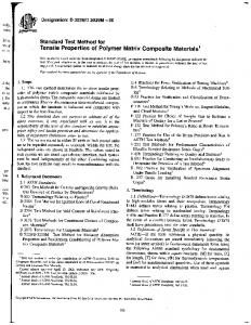
coefficient of thermal expansion (CTE) of the unidirectional C/C–SiC composites is proposed in this paper. The constraint is imposed on the allowable elastic modulus according to real applications. The micromechanical modeling approach, which provides the overall behavior of the composite through a finite element analysis of a unit cell model [6,7], is applied to obtain the CTE [8] and elastic modulus [9] of composites. The advantage of this approach is not only in obtaining global properties of the composite but also the behaviors that can be related to the composite microstructure. However, due to the complex multi-layered microstructure and large heterogeneity of multi-phase materials, a detailed unit cell finite element model of the unidirectional C/C–SiC composites involves a large number of elements. Generalization of the relationship between the microstructure and the overall properties of the composites using this finite element procedure is extremely difficult, especially in an optimization procedure. A new finite element mesh has to be rebuilt for each new situation and an iterative finite element analysis has to be carried out. This is extremely time consuming and computationally expensive. Thus, a hybrid approach is proposed in this paper by integrating the micromechanical model and artificial neural network for the identification of CTE and elastic modulus of the C/C–SiC composites. The artificial neural network has been extensively used in modeling composite material properties [10–13], especially for composite designing [14–16], as the relationship of the properties of the designed composite with its design parameters is very difficult to be represented as an explicit mathematical model. However, there is a lack of studies on applying the neural network in predicting the properties of C/C–SiC composites. The nonlinear and non-differentiable nature of the presented optimization problem induces difficulty in using classical deterministic approaches for solutions. To solve this nonlinear optimization problem, a particle swarm optimization (PSO) algorithm [17,18] is used. The PSO algorithm belongs to the category of swarm intelligence techniques. It has only a small number of parameters that need to be adjusted, and is easy to implement. Although the PSO algorithm has been applied to a wide range of engineering problems in the literature [19–22], few applications to C/C–SiC composites are known. In this study, a hybrid approach integrating the micromechanical model and artificial neural network is firstly proposed for the identification of CTE and elastic modulus of the unidirectional C/C–SiC composites. Predictions are compared with the results of a micromechanical model to assess the predictive capability of the proposed hybrid approach. The comparison shows that the forecast errors of the hybrid approach are inside the range of the relative fluctuations of testing samples. Although the neural network predictions partly agree with the micromechanical model, it is essential to improve the current neural network model in the future for an enhanced predicting capability. Then, a modified PSO algorithm is interfaced with the hybrid predictive model to minimize the CTE of a unidirectional C/C–SiC composite with six layers of alternating PyC and SiC matrix. The design variables are the thicknesses of matrix layers within the microstructure, and a constraint is imposed on the allowable elastic modulus. The classical PSO algorithm is modified to satisfy the constraints and the variable limits. The multi-stage penalty function method is adopted within PSO to satisfy the constraints, and the Harmony Search algorithm is used to deal with the particles that fly outside the variable boundaries. 2. Micromechanical Model of the Unidirectional C/C–SiC Composites 2.1. Unit Cell Model The architecture of the preform of unidirectional C/C–SiC composite consists of closely arranged fibers. The multi-layered PyC and SiC matrices are infiltrated within the porous fiber preforms by CVI process. Figure 1 shows the scanning electron microscope (SEM) photograph of a C/C–SiC composite [23], with the matrix consisting of alternate SiC (white color) and PyC (black color). It is clearly observed that the multi-layered matrices are distributed around the fibers. In addition, the pores are usually generated between adjacent fibers due to incomplete infiltration.

Materials 2016, 9, 222 Materials 2016, 9, 222 Materials 2016, 9, 222

3 of 16

Figure 1. 1. Scanning photographof ofaacarbon carbonfiber-reinforced fiber-reinforced multi-layered Figure Scanningelectron electronmicroscopy microscopy (SEM) (SEM) photograph multi-layered Figure 1. Scanning electron microscopy (SEM) photograph of a carbon fiber-reinforced multi-layered pyrocarbon-siliconcarbide carbidematrix matrix(C/C–SiC) (C/C–SiC) composite pyrocarbon-silicon composite[23]. [23]. pyrocarbon-silicon carbide matrix (C/C–SiC) composite [23].

For the CVI-processedcomposites, composites, the research research of indicated that For the CVI-processed of Chateau Chateauand andGélébart Gélébart[24] [24]has has indicated that For the CVI-processed composites,the the research of Chateau and Gélébart [24] has indicated that the residual pores after CVI process have an important influence on the mechanical behavior of thethe residual pores influence on onthe themechanical mechanicalbehavior behavior residual poresafter afterCVI CVIprocess processhave have an an important important influence of of composites. Thus, for an accurate simulation of the material behavior, one must carefully introduce composites. Thus, materialbehavior, behavior,one onemust mustcarefully carefully introduce composites. Thus,for foran anaccurate accuratesimulation simulation of the material introduce these manufacturing flaws in a computing scheme. However, in the present study, a highly idealized these manufacturing However,in inthe thepresent presentstudy, study,a ahighly highly idealized these manufacturingflaws flawsininaacomputing computing scheme. scheme. However, idealized unit cell model is employed. Our purpose is to use this idealized model to develop a numerical unit model is employed. purpose to this use idealized this idealized model to develop a numerical unit cellcell model is employed. OurOur purpose is toisuse model to develop a numerical scheme scheme in an efficient manner for optimizing the thermal-elastic properties of composites. Thus, the scheme in an efficient for optimizing the thermal-elastic properties of composites. the in an efficient manner formanner optimizing the thermal-elastic properties of composites. Thus, theThus, presented presented research in this paper puts more emphasis on creating a validated and expandable presented research in this paper puts more emphasis on creating a validated and expandable research in thisscheme. paper puts moreitemphasis creating validated expandabledesign optimization optimization However, should be on noted that fora an accurateand microstructure of the optimization scheme. However, it should befor noted that for anmicrostructure accurate microstructure design of the scheme. However, it should be noted that an accurate design of the C/C–SiC composites, the pores and fiber positions must be carefully captured and modeled.C/C–SiC To do C/C–SiC composites, thefiber pores and fiber positions must be carefully captured and To X-ray do composites, the pores and positions must and modeled. Tomodeled. do this, the this, the X-ray micro-computed tomography isbeancarefully effectivecaptured tool that has shown its applicability in the this, the X-ray micro-computed tomography is an effective tool that has shown its applicability in the micro-computed tomography is an effective thatstudy, has shown its applicability in the work of Chateau work of Chateau and Gélébart [24]. In our tool future for a high-quality optimization of C/C–SiC work of Chateau Gélébartstudy, [24]. In our future study,optimization for a high-quality optimization of C/C–SiC and Gélébart [24]. Inand our for a high-quality offiber C/C–SiC composites, a more composites, a more realfuture unit cell including the heterogeneous pore and distributions would be composites, a more real unit cell including the heterogeneous pore and fiber distributions would be real unit cell including the heterogeneous pore and fiber distributions would be carefully modeled. carefully modeled. carefully modeled. InIn this paper, a unidirectional compositewith withsix sixlayers layersofofalternating alternating PyC and this paper, a unidirectionalC/C–SiC C/C–SiC composite PyC and SiCSiC is is In this paper, a unidirectional C/C–SiC composite with six layers of alternating PyC and SiC is considered a case study. A geometrical of the cell is displayed in Characteristic Figure 2a. considered as aascase study. A geometrical model model of the unit cell unit is displayed in Figure 2a. considered as a case study. A geometrical model of the unit f cell is displayed in Figure 2a. Characteristic geometric parameters unit cell arefiber given: φ is fiber d1–d6 are of geometric parameters of the unit cell of arethe given: ϕ f is diameter anddiameter d1 –d6 areand thicknesses Characteristic geometric parameters of the unit cell are given: φf is fiber diameter and d1–d6 are thicknesses of the matrix layers. The six layers of matrices are alternating PyC and SiC material layers the matrix layers. The six layers of matrices are alternating PyC and SiC material layers (denoted thicknesses of the matrix layers. The six layers of matrices are alternating PyC and SiC material layers as PyC/SiC/PyC/SiC/PyC/SiC). cellis then model is thenusing meshed using the 3-D as (denoted PyC/SiC/PyC/SiC/PyC/SiC). The unitThe cell unit model the 3-D twenty-node, (denoted as PyC/SiC/PyC/SiC/PyC/SiC). The unit cell modelmeshed is then meshed using the 3-D twenty-node, thermal-structural coupled element (SOLID 96) of ANSYS finite element software, thermal-structural coupled element (SOLID 96) of ANSYS finite element software, as depicted twenty-node, thermal-structural coupled element (SOLID 96) of ANSYS finite element software, in as depicted in Figure 2b. Figure 2b. as depicted in Figure 2b.

(a) (a)

(b) (b)

Figure 2. Unit cell of the unidirectional C/C–SiC composites: (a) Geometrical model; (b) Finite element model. Figure 2. Unit cell of the unidirectional C/C–SiC composites: (a) Geometrical model; (b) Finite element model. Figure 2. Unit cell of the unidirectional C/C–SiC composites: (a) Geometrical model; (b) Finite element model.

3 3

Materials 2016, 9, 222

4 of 16

2.2. Computation of the Elastic Modulus In this study, a strain energy-based finite element approach is applied to evaluate effective elastic properties. It is assumed that each unit cell in the composites has the same deformation mode and that there is no separation or overlap between neighboring unit cells. Therefore, the periodic boundary conditions (PBC) [25–27] must be applied to the unit cell model. The PBC can be applied using nodes coupling (CP) and constraint equations (CE) defining in ANSYS. Then, the explicit formulations between the stiffness matrix coefficients and the strain energy of the unit cell model under specific loadings are derived. The detailed description of this method can be found in [28,29]. Here, only a basic introduction is presented. In the elastic regime, the macroscopic behaviors of the unit cell can be characterized by the effective stress tensor σ and strain tensor ε over the homogeneous equivalent model. They are interrelated by the effective, also termed homogenized, stiffness matrix C H . σ “ CH ε

(1)

ş ş where σ “ 1{V Ω σdΩ, ε “ 1{V Ω εdΩ, and V is the volume of the unit cell. Consider the case of 3-D orthotropic materials; Equation (1) corresponds to » — — — — — — — –

σ11 σ22 σ33 σ12 σ23 σ31

fi

»

ffi — ffi — ffi — ffi — ffi “ — ffi — ffi — fl –

H C1111 H C1122 H C1133 0 0 0

H C1122 H C2222 H C2233 0 0 0

H C1133 H C2233 H C3333 0 0 0

0 0 0 H C1212 0 0

0 0 0 0

0 0 0 0 0

H C2323 0

fi » ffi — ffi — ffi — ffi — ffi — ffi — ffi — fl –

H C3131

ε11 ε22 ε33 ε12 ε23 ε31

fi ffi ffi ffi ffi ffi ffi ffi fl

(2)

The strain energy related to the microstructure is equal to: ż E“

Ω

1 pσ ε ` σ22 ε 22 ` σ33 ε 33 ` σ12 ε 12 ` σ23 ε 23 ` σ31 ε 31 q dΩ 2 11 11

1 “ pσ11 ε11 ` σ22 ε22 ` σ33 ε33 ` σ12 ε12 ` σ23 ε23 ` σ31 ε31 q V 2

(3)

With the help of specific loadings, the combination of Equation (2) and Equation (3) can be used to deduce the effective stiffness matrix C H for the unit cell. Suppose a unit initial strain is imposed in ´p1q

the y1 direction; i.e., ε “ p1 0 0 0 0 0qT . Note that the superscript (1) represents the first load case. The corresponding average stress is then obtained by Equation (2): ´p1q

H H H σ “ pC1111 C1122 C1133 0 0 0q

By replacing strain energy:

´p1q

σ

and

´p1q

ε

T

(4)

into Equation (3), one obtains the following expression of the Ep1q “

1 ´p1q´p1q 1 H σ ε V “ C1111 V 2 2

(5)

H The matrix coefficient C1111 can be derived: H C1111 “ 2Ep1q {V

(6)

In the same way, demonstrations can be made for other coefficients, and all the results are summarized in Table 1. The elastic properties can be derived by inversing the elastic matrix. In practice, the considered unit cell will be discretized into a finite element model on which the initial strain will be imposed to evaluate the strain energy.

Materials 2016, 9, 222

5 of 16

Table 1. Different loadings and the coefficients of elastic matrix. Load Case

Loadings

Effective Coefficients of Elastic Matrix

1

´p1q

H C1111 “ 2Ep1q {V

2

´p2q

H C2222 “ 2Ep2q {V

3

´p3q

H C3333 “ 2Ep3q {V

4

´p4q

H C1212 “ 2Ep4q {V

5

´p5q

H C2323 “ 2Ep5q {V

6

´p6q

H C3131 “ 2Ep6q {V

7

´p7q

H H {2 ´ C H {2 C1122 “ Ep7q {V ´ C1111 2222

8

´p8q

H H {2 ´ C H {2 C2233 “ Ep8q {V ´ C2222 3333

9

´p9q

H H {2 ´ C H {2 C1133 “ Ep9q {V ´ C1111 3333

ε “ p1 0 0 0 0 0qT ε “ p0 1 0 0 0 0qT ε “ p0 0 1 0 0 0qT ε “ p0 0 0 1 0 0qT ε “ p0 0 0 0 1 0qT ε “ p0 0 0 0 0 1qT ε “ p1 1 0 0 0 0qT ε “ p0 1 1 0 0 0qT ε “ p1 0 1 0 0 0qT

2.3. Computation of the CTE Here, the CTE of the composites is determined by finite element computation of the unit cell with specific structural and thermal loadings [30]. As shown in Figure 1a, along the planes x1 = 0, x2 = 0, and x3 = 0, the model is restricted to move in the x1 , x2 , and x3 directions. Planes x1 = l1 , x2 = l2 , and x3 = l3 are free to move but have to remain planar in a parallel way to preserve the compatibility with adjacent cells. Suppose the deformation of the unit cell is caused by a temperature rise of ∆T. During the deformation, xi = li becomes xi = li + ∆li , and the displacement, ∆li , can be determined from the finite element analysis. The CTE in direction i then corresponds to αi “

∆li li ∆T

(7)

2.4. Experiment To test the accuracy of the micromechanical model, three samples of the unidirectional C/C–SiC composites with different layer thicknesses were fabricated. The fiber preforms were close-packed 1K T-300 carbon fiber yearns from Nippon Toray (Tokyo, Japan). The multi-layered PyC and SiC matrix were deposited by CVI process using butane and methyltrichlorosilane (MTS) as the reactive materials in School of Material, Northwestern Polytechnical University, Xi’an, PR China. The infiltration condition of PyC was: temperature 960 ˝ C, pressure 5 KPa, Ar flow 200 mL/min, butane flow 15 mL/min. The infiltration condition of SiC was: temperature 1000 ˝ C, pressure 5 KPa, H2 flow 350 mL/min, Ar flow 350 mL/min, and the molar ratio of H2 and MTS of 10. Different layer thicknesses are obtained by controlling the infiltration time. The detailed illustration for the above process can be found in [3]. Elastic constants and CTEs of each material phase were taken from [3] and listed in Table 2. In this study, three groups of layers thicknesses were designed by controlling the infiltration time and are listed in Table 3. The fiber volume fractions of three samples were 19.7%, 19.7%, and 19.1%, respectively. Here, it should be noted that there indeed exists discrepancy between the designed thickness and the measured thickness, due to the complexity of the CVI process. However, since the purpose of this experiment is to verify the micromechanical model in an efficient manner, the discrepancy between the designed and true thickness values is neglected to simplify the experiment implementation (i.e., avoid the complex measurement of layer thicknesses in the SEM microphotographs).

Materials 2016, 9, 222

6 of 16

Table 2. Properties for each material phase. Material Phase

E11 GPa

E33 GPa

G12 GPa

G23 GPa

v12

v23

α11 10´6 /˝ C

α33 10´6 /˝ C

T-300 carbon fiber pyrolytic carbon silicon carbide

22 12 350

220 30 –

7.75 2.0 145.8

4.8 4.3 –

0.42 0.4 0.2

0.12 0.12 –

8.85 1.8 4.5

´0.7 – –

Table 3. Comparison of measured and predicted modulus and coefficients of thermal expansion (CTEs).

Sample A B C

Layer Thickness (µm)

Modulus E33 (GPa)

CTE α33 (10´6 /˝ C)

CTE α11 (10´6 /˝ C)

d1

d2

d3

d4

d5

d6

Model

Test

Model

Test

Model

Test

0.5 0.5 1.0

1.0 0.5 0.5

0.5 0.5 1.0

1.0 1.0 0.5

0.5 1.0 1.0

1.0 1.0 0.5

256.2 225.5 175.1

226.1 200.1 155.8

3.753 3.646 3.421

3.309 3.235 3.021

4.356 4.242 4.009

3.893 3.847 3.630

Uniaxial tensile tests were conducted at room temperature to obtain the longitudinal tensile modulus of the composites. Quasi-static tension tests were performed on a DNS-100 electronic universal testing system (CIMACH, Changchun, China). To measure the longitudinal and transverse CTEs of composites, DIL 402C dilatometer made by NETZSCH Company (Selb, Germany) was employed. Predictions based on the micromechanical model were compared with experimental data. The diameter of T-300 carbon fiber is 7.0 µm. The modulus and CTEs obtained in the previous tests for composite samples (denoted as A, B, and C) with different layer thicknesses, listed in Table 3, were chosen for comparison. Table 3 shows the comparison of measured and predicted modulus and CTEs for the various composite samples. It can be seen that the predicted results coincide well with the experimental data. The comparative results may highlight the predictive capacity of the proposed micromechanical model for predicting the elastic modulus and CTEs of unidirectional C/C–SiC composite. However, it should be pointed out that because rudimental cavities generated within the composite for the emission of large infiltrated by-products during the infiltration are not considered in this paper; thus, the modulus and CTEs computed numerically by the present model are larger than the experimental results. 3. Optimization Problem In this paper, a unidirectional C/C–SiC composite consisting of six layers of matrices made up of alternate PyC and SiC is used as a case study. In high temperature environments, one of the common requirements is to use C/C–SiC composites with low thermal expansion behaviors and high elastic modulus. Thus, the objective of this study is to minimize the CTE of composites with elastic modulus constraints. The optimization problems given in the present study include two cases, which include, respectively, the minimization of the longitudinal and transverse CTEs. A constant fiber volume fraction of 30% is defined for the composites. Therefore, an equality constraint is imposed on the sum of the thicknesses of matrix layers. Note that in order to simplify the programming implementation, this equality constraint is transferred to inequality constraints, as illustrated in Equations (8) and (9) (∆ = 0.01). D0 is a constant derived from the fiber volume fraction. In this study, D0 is equal to 5.168 for a 30% fiber volume fraction. In addition, since the load-bearing capability of C/C–SiC composite structures in industrial applications is primarily related to the tensile modulus E33 , another constraint is imposed on the allowable value of E33 according to the real applications.

Materials 2016, 9, 222

7 of 16

Mathematically, the optimization problems can be formulated as follows: Minimize α33 pXq X “ pd1 , d2 , ..., d6 q $0.2 ď di ď 1.0, 1 ď i ď 6 ’ 200.0 ´ E33 pXq ď 0 & ř Subject to d6 ` 2 5i“1 di ´ pD0 ` ∆q ď 0 ’ % pD ´ ∆q ´ d ´ 2ř5 d ď 0 0 6 i “1 i Minimize α11 pXq X “ pd1 , d2 , ..., d6 q 0.2 $ ď di ď 1.0, 1 ď i ď 6 ’ 200.0 ´ E33 pXq ď 0 & ř Subject to d6 ` 2 5i“1 di ´ pD0 ` ∆q ď 0 ’ % pD ´ ∆q ´ d ´ 2ř5 d ď 0 0 6 i “1 i

(8)

(9)

The design variables are the thicknesses of the matrix layers. The fiber diameter ϕ f is 7.0 µm. Elastic constants and CTEs of each material phase are listed in Table 2. The upper bound of matrix layer thickness is 1.0 µm. The lower bound of thickness of matrix is set to 0.2 µm for reducing the complexity of the fabrication process. 4. Back Propagation (BP) Neural Network Model The proposed micromechanical modeling approach has shown favorable predicting capability for the thermal-elastic properties of C/C–SiC composites. However, a high computational cost would be induced due to the large number of elements of the complex multi-layered microstructure. Especially in an optimization procedure, for each new situation, a finite element mesh has to be rebuilt and an iterative finite element analysis has to be carried out. This is extremely time consuming and computationally expensive. The most important benefit of an artificial neural network is the high computing efficiency. Therefore, in this study a hybrid approach integrating the micromechanical model and an artificial neural network is proposed for the determination of the CTE and elastic modulus of the C/C–SiC composites. The BP neural network has the powerful ability of non-linear interpolation to obtain the mathematical mapping reflecting the internal law of the experimental data. In this study, a four-layer BP neural network containing one input layer, two hidden layers and one output layer is developed to construct the mapping between the layer thicknesses and the thermal-elastic properties of unidirectional C/C–SiC composites. Every neural network has exactly one input layer and one output layer. So we only need to determine the number of hidden layers. Heaton [31] summarized the capabilities of neural network architectures with various hidden layers: the hidden layer is not needed if the function is linearly separable; one hidden layer can approximate any function that contains a continuous mapping from one finite space to another; two hidden layers can represent an arbitrary decision boundary to arbitrary accuracy with rational activation functions and can approximate any smooth mapping to any accuracy. Therefore, two hidden layers are used in this study. Although two hidden layers increases the computational cost, their capability of representing functions with any kind of shape provides a promising tool for our further study. Figure 3 illustrates the BP neural network architecture used in this study. The network contains three parts: one input layer having six neurons related to the layer thicknesses; two hidden layers with 20 neurons for each one, and one output layer having three neurons representing the transverse and longitudinal CTEs α11 and α33 and the modulus E33 . There are many general methods for determining the number of neurons in the hidden layers. However, these rules just provide a starting point for

Materials 2016, 9, 222

8 of 16

users to consider. For the problem considered in this study, one of the commonly-used rules gives an approximate range for the number of neurons in a hidden layer: n“

?

ni ` n o ` α

(10)

where n is the number of neurons in the hidden layer, ni is the number of neurons in the input layer, no is the number of neurons in the output layer, α is a constant from 1 to 10. According to the empirical equation, in this study the number of neurons in the hidden layer is between 4 and 13. Considering a BP neural network with more neurons in the hidden layer can give a higher precision solution [32]; the Materials 9, 222 number2016, of neurons in the hidden layer is finally selected as 20 in this paper.

Figure 3. 3. Back Back Propagation Propagation (BP) (BP) neural neural network network architecture architecture used in this study. Figure

In the network, the total input, injj,, received received by by the the jth jth neuron neuron in in the the hidden hidden layer layer from all of the neurons in the preceding layer is: N ÿ N ininj “   ωijxxi (11) (11) j ij i j 0 j“ 0

where N is the number of inputs to the jth neuron in the hidden layer, xi is the input from the ith neuron in the preceding layer, and wijij is is the the connection connection weight weight from from the the ith ith neuron in the forward layer to the jth neuron in the hidden layer. layer. The neuron then processes the input through a transfer function fs as below to produces its output outjj:: in j ` ˘ 1 ´ e´ in out j “ f s in j “ 1  e ´ (12) out j  fs  inj   1 ` e in in j (12) j

1 e

j

Before the above BP neural network system can be used to predict the thermal-elastic properties of Before theitabove BPtrained neural by network system can from be used predict the thermal-elastic properties the composite, must be the data obtained the to micromechanical model. The connection of the composite, it must be trained by the data obtained from the micromechanical model. The weight wij will be calculated by minimizing the error between the predictive value and the actual value connection weight w ij will be calculated by minimizing the error between the predictive value and during the training process. Details about the training process will be discussed in the following section. the actual value during the training process. Details about the training process will be discussed in 4.1. following Generationsection. of Training Data the In this study, the training data are obtained from the micromechanical computations. In order to 4.1. Generation of Training Data reflect the inner relationship between the thermal-elastic properties and the matrix layer thicknesses, a In this study, the training obtained from the micromechanical computations. In order full factorial experimental designdata is noare doubt an excellent idea. However, the full factorial experimental to reflect the that inner relationship between the thermal-elastic properties and matrix design means a large number of computations (15,625 in this study) should be the taken, whichlayer will thicknesses, a full factorial experimental is no doubt an excellent idea. However, the full obviously consume much time. Therefore,design the Taguchi orthogonal array [33] which suggests using factorial experimental design means that a large number of computations (15,625 in this study) should be taken, which will obviously consume much time. Therefore, the Taguchi orthogonal array [33] which suggests using less simulation to find out the relationship between parameters is employed in this study. 25 samples designed by the L25 orthogonal array as well as another 35 samples randomly

Materials 2016, 9, 222

9 of 16

less simulation to find out the relationship between parameters is employed in this study. 25 samples designed by the L25 orthogonal array as well as another 35 samples randomly generated by computer, 60 samples in sum, are used to train the designed network. 4.2. Neural Network Training Materials 2016, 9, 222

During the training process, the connection weights should be calculated by minimizing the mean square error network predictions and training data. Equation (13) [31] isvalues used to the random, andbetween then they are iteratively updated until convergence to the certain byupdate using the connection weights iteratively. At the beginning of the training, the weights are given at random, gradient descent method. and then they are iteratively updated untilnew convergence to the certain values by using the gradient ij  ijold  ij descent method. ωijnew “ ωijoldE ` ∆ωij (13) ij   BE out j (13)   ∆ωij “ ´η ij out j Bωij −4. η is the learning rate parameter controlling the where E is the mean square error and is set as 1 × 10´ where E is the mean square error and is set as 1 ˆ 10 4 . η is the learning rate parameter controlling the stability and rate of convergence of the network, which is usually a constant between 0 and 1 and is stability and rate of convergence of the network, which is usually a constant between 0 and 1 and is chosen to be 0.01 in this study. Totally, the number of the connection weights to be identified is 580. chosen to be 0.01 in this study. Totally, the number of the connection weights to be identified is 580. 5 The training process takes about 1200 s of CPU time on HP personal workstation for 4.0 × 105 The training process takes about 1200 s of CPU time on HP personal workstation for 4.0 ˆ 10 training iterations. Figure 4 gives the variation curve of the mean square error with the iteration of training iterations. Figure 4 gives the variation curve of the mean square error with the iteration of connection weights (according to Equation (13)). It can be observed that with the updating of the connection weights (according to Equation (13)). It can be observed that with the updating of the connection weights, the mean square error has been gradually declined and converged to 1 × 10´−44. connection weights, the mean square error has been gradually declined and converged to 1 ˆ 10 . The mathematic mapping between the layer thicknesses and the CTE and elastic modulus is then The mathematic mapping between the layer thicknesses and the CTE and elastic modulus is then stored in the trained net. The mathematic function can be expressed as: stored in the trained net. The mathematic function can be expressed as:







S i   ´ fl ÿ (14) ÿw1 X ¯¯¯  w3 fs´ÿ  w2 fs ´ S piq “ f l w3 f s w2 f s w1 X (14) where S(i) (i = 1, 2, 3) represents the CTE and elastic modulus; X = [x1, x2, x3, x4, x5, x6] is the vector where S(i) of (i = 1, thickness 2, 3) represents CTE and elastic X =transfer [x1 , x2 , xfunction x6 ] is thehidden vector consisting the valuesthe of six matrix layers; modulus; fl is the linear 3 , x4 , x5 , between consisting theoutput thickness values of six matrixfunction layers; fbetween transfer function between hidden layer 2 andofthe layer; fs is the transfer the input layer and hidden layer 1, as l is the linear layeras 2 and the output fs is function the input layer and hidden layerlayer 1, as well hidden layers 1layer; and 2; w1the , w2transfer , w3 represent thebetween connection weights between the input well hidden as hidden layers 1 and 2;layer w1 , w21, and w3 represent the connection weights between layer and and layer 1, hidden hidden layer 2, and hidden layer 2 andthe theinput output layer, hidden layer 1, hidden layer 1 and hidden layer 2, and hidden layer 2 and the output layer, respectively. respectively.

Figure Figure 4. 4. Training Training process process of of the the network. network.

4.3. 4.3. Neural Neural Network Network Testing Testing In order to to demonstrate demonstratethe theability abilityofofa aneural neural network system generalize training data, In order network system to to generalize thethe training data, the the neural network is used to estimate the modulus and CTEs of the input design parameter neural network is used to estimate the modulus and CTEs of the input design parameter combination. combination. of layer thicknesses randomly generated byused computer (not used in the Twenty groupsTwenty of layergroups thicknesses randomly generated by computer (not in the training process) training process) are used in the testing and are listed in Table 4. are used in the testing and are listed in Table 4.

Materials 2016, 9, 222

10 of 16

Table 4. 20 groups of layer thicknesses used in the testing. Layer Thickness (µm)

Nos. 1 2 3 4 5 6 7 8 9 10 11 12 13 14 15 16 17 18 19 20

d1

d2

d3

d4

d5

d6

0.2610 0.4644 0.4830 0.5711 0.7319 0.9353 0.8524 0.9357 0.7467 0.7100 0.7460 0.7125 0.8549 0.3470 0.8721 0.8748 0.9856 0.9970 0.8432 0.2610

0.5662 0.8772 0.4023 0.3550 0.7946 0.4803 0.8761 0.5894 0.7546 0.6951 0.2228 0.9604 0.4947 0.7968 0.5665 0.3878 0.6024 0.2374 0.7456 0.7432

0.2480 0.2833 0.4673 0.9901 0.5799 0.8645 0.7855 0.7152 0.2069 0.9807 0.2224 0.9500 0.8741 0.8577 0.3505 0.8542 0.3441 0.4513 0.8845 0.4422

0.3919 0.2048 0.7826 0.3457 0.3282 0.8642 0.8279 0.5864 0.8498 0.4282 0.9292 0.2565 0.7923 0.3749 0.2041 0.8348 0.6426 0.5714 0.9966 0.7643

0.9195 0.2793 0.4900 0.3629 0.7503 0.6044 0.2979 0.2819 0.8370 0.9433 0.3738 0.9891 0.8863 0.9302 0.4703 0.5209 0.7592 0.9666 0.4197 0.6063

0.3899 0.6328 0.6968 0.6663 0.7479 0.6487 0.7361 0.4140 0.5739 0.2059 0.2794 0.4261 0.5873 0.6073 0.9845 0.4124 0.3716 0.6571 0.7483 0.7591

Table 5 shows the comparison between the neural network prediction and micromechanical computation. The forecast error is defined as: F e “ pS p ´ Sm q {Sm

(15)

where Fe represents the forecast error of the prediction system. S p is the result of neural network prediction, and Sm stands for the result of micromechanical computation. Table 5. Comparison between the neural network prediction and micromechanical computation.

Nos. 1 2 3 4 5 6 7 8 9 10 11 12 13 14 15 16 17 18 19 20

CTE α33 (10´5 /˝ C) Sp

Sm

0.2978 0.3114 0.3256 0.3276 0.3336 0.3711 0.3860 0.3514 0.3460 0.3461 0.3333 0.3560 0.3684 0.3534 0.3403 0.3343 0.3261 0.3196 0.3891 0.3415

0.3115 0.3218 0.3390 0.3164 0.3451 0.3581 0.3681 0.3392 0.3584 0.3338 0.3226 0.3438 0.3552 0.3409 0.3283 0.3456 0.3430 0.3311 0.3715 0.3592

Fe

CTE α11 (10´5 /˝ C) (%)

´4.40 ´3.24 ´3.96 3.54 ´3.33 3.62 4.88 3.58 ´3.47 3.68 3.31 3.56 3.73 3.67 3.64 ´3.27 ´4.91 ´3.47 4.76 ´4.93

Sp

Sm

0.4019 0.4637 0.4520 0.4133 0.4057 0.4091 0.4224 0.4158 0.4345 0.4014 0.4234 0.4065 0.4260 0.3931 0.4258 0.4046 0.4280 0.4321 0.4476 0.4475

0.4163 0.4459 0.4369 0.4306 0.4194 0.4234 0.4358 0.4296 0.4188 0.3871 0.4380 0.3927 0.4118 0.4085 0.4412 0.4213 0.4127 0.4163 0.4319 0.4290

Fe

Modulus E33 (GPa) (%)

´3.46 3.99 3.47 ´4.01 ´3.25 ´3.36 ´3.06 ´3.20 3.74 3.69 ´3.35 3.51 3.45 ´3.78 ´3.49 ´3.98 3.69 3.80 3.62 4.29

Sp

Sm

Fe (%)

211.031 243.368 228.380 190.841 202.234 215.198 225.689 206.528 237.316 173.465 242.812 191.179 202.535 211.295 227.551 197.096 213.942 193.728 236.370 224.879

220.368 251.517 236.248 200.759 209.252 207.463 233.787 213.309 228.926 179.566 233.045 185.067 196.341 203.589 218.387 204.209 206.342 187.862 228.074 232.518

´4.24 ´3.24 ´3.33 ´4.94 ´3.35 3.73 ´3.46 ´3.18 3.66 ´3.40 4.19 3.30 3.15 3.78 4.20 ´3.48 3.68 3.12 3.64 ´3.29

Materials 2016, 9, 222

11 of 16

It is seen that the forecast errors of α11 and α33 are respectively inside the ranges of (´4.01%, 4.29%) and ˙(´4.93%, 4.88%). of Sm is defined as ˆ ˆ Here, mif the relative ˙ mfluctuation m m m m m m m ´ Smax ` Smin { Smax ` Smin , Sm ´ Smax ` Smin { Smax ` Smin ), we can easily obtain ( Smin max 2 2 2 2 the relative fluctuations of α11 and α33 within the 20 groups of testing samples: (´10%, 10%) and (´11%, 11%). The above results clearly indicate that both the forecast errors of α11 and α33 fall in the range of fluctuations. Therefore we want to emphasize that although the neural network predictions partly agree with the micromechanical model, the improvement of the current neural network is still needed in future for an enhanced predicting capability. Possible refining approaches include supplementing adequate training samples with a wider range and optimizing the neural network. The running time of the prediction system is sharply decreased compared to that of the micromechanical analysis. The average running time of one micromechanical computation (including 12 finite element analyses) is about 2500 s and that of neural network prediction system is only about 0.001 s. 5. Particle Swarm Optimization Algorithm In a PSO algorithm, each individual of the swarm is considered as a flying particle in the design space that has a position and a velocity. The particles remember the best position that they have seen during the flying. Members of a swarm remember the location where they had their best success and communicate good positions to each other, then update their own position and velocity based on these good positions as follows: ´ ¯ ´ ¯ Vik`1 “ ωVik ` c1 r1 Pik ´ Xik ` c2 r2 Pgk ´ Xik

(16)

Xik`1 “ Xik ` Vik`1

(17)

where Vi and Xi represent the velocity and the position of the ith particle, respectively (the subscripts k and k + 1 refer to the recent and the next iterations, respectively). Pi is the best previous position of the ith particle and Pg is the best global position among all the particles in the swarm. ω is the inertia weight controlling the impact of the previous history of velocities on the current velocity and is set to 0.875 in this study. c1 and c2 are acceleration constants indicating the stochastic acceleration terms which pull each particle towards the best position attained by the particle or the best position attained by the swarm. In this work, c1 = 2 and c2 = 2 are chosen. r1 and r2 are two random numbers between 0 and 1. Most optimization problems include the problem-specific constraints and the variable limits. For the present optimization, the problem-specific constraint is the elastic modulus, and the variable limits are design bounds of the thicknesses of matrix layers. If the particle flies out of the variable boundaries, the solution cannot be used even if the problem-specific constraint is satisfied, so it is essential to make sure that all of the particles fly inside the variable boundaries, and then to check whether they violate the problem-specific constraint. 5.1. Harmony Search Scheme: Handling the Variable Limits A method introduced by Li et al. [34] dealing with the particles that fly outside the variable boundaries is used in the present study. This method is derived from the harmony search (HS) algorithm. In the HS algorithm, the harmony memory (HM) stores the feasible vectors, which are all in the feasible space. The harmony memory size determines how many vectors can be stored. A new vector is generated by selecting the components of different vectors randomly in the harmony memory. Undoubtedly, the new vector does not violate the variables boundaries. When it is generated, the harmony memory will be updated by accepting this new vector if it gets a better solution and deleting the worst vector. Similarly, the PSO algorithm stores the feasible and “good” vectors (particles) in the pbest swarm, as does the harmony memory in the HS algorithm. Hence, the vector (particle) violating the variable boundaries can be generated randomly again by such a strategy: if any component of

Materials 2016, 9, 222

12 of 16

Materials 2016, 9, 222

the current particle violates its corresponding boundary, then it will be replaced by selecting the replaced by selecting the corresponding component of the particle from pbest swarm randomly. To corresponding component of the particle from pbest swarm randomly. To highlight the presentation, a highlight the presentation, a schematic diagram is given in Figure 5 to illustrate this strategy. schematic diagram is given in Figure 5 to illustrate this strategy.

Figure 5. Illustration of the variable limits handling strategy. strategy.

5.2. Penalty Penalty Functions Functions Method: Method: Handling Handling the the Problem-Specific Problem-Specific Constraints Constraints 5.2. The most constraints is the useuse of aofpenalty function. The The most common common method methodofofhandling handlingthe the constraints is the a penalty function. constrained problem is transformed to an unconstrained one, by penalizing the constraints and The constrained problem is transformed to an unconstrained one, by penalizing the constraints building a single objective function. Hence, the optimization problem becomes oneone of minimizing the and building a single objective function. Hence, the optimization problem becomes of minimizing objective function andand thethe penalty together. multi-stage penalty penalty the objective function penalty together.InInthis thispaper, paper,aa non-stationary, non-stationary, multi-stage function method implemented by Parsopoulos and Vrahatis [35] is adopted for constraint handling function method implemented by Parsopoulos and Vrahatis [35] is adopted for constraint handling with PSO. PSO. The The penalty penalty function function is is with

F  X   f  X   h  k  H  X  , X  S  Rn

(18) (18)

F pXq “ f pXq ` h pkq H pXq , X P S Ă Rn

where f(X) is the original objective function to be optimized. h(k) is a penalty value which is modified where f(X) is the original objective function to be optimized. h(k) is a penalty value which ? is modified h k “ kk.. H(X) is aa according to to the the algorithm’s algorithm’s current current iteration iteration number number kk and and isisusually usuallyset settotoh pkq according penalty penalty factor factor defined defined as: as: m ÿ H pXq “ mθ pqi pXqq qi pXqγ p qqi ipXXqq (19) H  X  i“ (19) 1   qi  X   qi  X 



i 1

where qi (X) is a relative violated function of the constraints, which is defined as qi (X) = max {0, gi (X)} where qi(X) is a relative violated function of the constraints, which is defined as qi(X) = max {0, gi(X)} (Note that gi (X) is the constraint), θ pqi pXqq is an assignment function, and γ pqi pXqq is the power of qi Xthe following qi X function: (Note that gfunction. i(X) is theRegarding constraint), is an assignment function, and is the power the penalty the[10], values are used for thepenalty ă 1, then γ pqi pXqq “ 1; the [10], the following values are used for the penalty function: If i pXq ofqthe penalty function. Regarding otherwise γ pqi pXqq “ 2; If qi X  1 , then  qi X  1 ; ă 0.001, then θ pqi pXqq “ 10; If qi pXq else if qi pXq ďqi0.1, X then  2 θ; pqi pXqq “ 20; otherwise else if qi pXq ď 1, then θ pqi pXqq “ 100; qi X  10 ; If qi X  θ0.001 , then “ 300. otherwise pq pXqq

  

 

  

  

  

   else if q  X   0.1 , then   q  X   20 ; 6. Results   q  X illustrated  100 ; in Section 3 are implemented by using the proposed hybrid else if  X   1 , thenproblems Theq optimization approach   qPSO otherwiseand  X algorithm.   300 . For all the optimization problems, a population of 50 particles is used. The stopping criterion can be defined based on the number of iterations without an update in the  

i

i

i

i

i

i

best values of the swarm or the number of iterations the algorithm executes. Although the latter is 6. Results not a real physical stopping criterion, it is quite easy in programming implementation and hence is The optimization problems illustrated in Section 3 are implemented by using the proposed hybrid approach and PSO algorithm. For all the optimization problems, a population of 50 particles is used. The stopping criterion can be defined based on the number of iterations without an update 12

Materials 2016, 9, 222 Materials 2016, 9, 222

13 of 16

in the best values of the swarm or the number of iterations the algorithm executes. Although the latter is not a real physical stopping criterion, it is quite easy in programming implementation and hence is widely used in PSO algorithms. In this work, maximum number of iterations is limited to and 100 widely used in PSO algorithms. In this work, the the maximum number of iterations is limited to 100 and is adopted asstopping the stopping criterion. is adopted as the criterion. Figure 6 provides the convergence rates of of the the optimization optimization procedure procedure for for minimizing minimizing the the Figure 6 provides the convergence rates longitudinal CTE. The algorithm achieves the best solution after about 50 iterations. The longitudinal longitudinal CTE. The algorithm achieves the best solution after about 50 iterations. The longitudinal −6˝ CTE has hasbeen beeneffectively effectivelyreduced reduced 2.89 ×´ 106 / /°C. Theconvergence convergence design variables during CTE to to 2.89 ˆ 10 C. The ofof thethe design variables during the the iterations is shown in Figure 7. It is observed that the thicknesses of the first (PyC) matrix layer iterations is shown in Figure 7. It is observed that the thicknesses of the first (PyC) matrix layer increases increases to its higher bound. third and last (PyC) matrix layers both reachvalues median values to its higher bound. The third The (PyC) and(PyC) last (PyC) matrix layers both reach median between between the lower and higher bounds. The second (SiC), fourth (SiC), and fifth (PyC) matrix layers the lower and higher bounds. The second (SiC), fourth (SiC), and fifth (PyC) matrix layers all iterate all iterate to values near the lower bound. The final optimized thicknesses are to values near the lower bound. The final optimized thicknesses are 0.999/0.259/0.557/0.215/0.276/ 0.999/0.259/0.557/0.215/0.276/0.525 μm. 0.525 µm.

Figure for minimizing minimizing the the longitudinal longitudinal CTE. CTE. Figure 6. 6. Convergence Convergence rates rates of of the the optimization optimization procedure procedure for

CTE. Figure 7. Convergence of the design variables for minimizing the longitudinal longitudinal CTE.

Figure 88 provides provides the the convergence convergence rates rates of of the the optimization optimization procedure procedure for for minimizing minimizing the the Figure transverse CTE. CTE.The Thealgorithm algorithmachieves achieves best solution after about 80 iterations. The transverse transverse thethe best solution after about 80 iterations. The transverse CTE −6/°C. The convergence of the design variables during CTE has been effectively reduced to 4.09 × 10 ´ 6 ˝ has been effectively reduced to 4.09 ˆ 10 / C. The convergence of the design variables during the the iterations is shown in Figure 9. is It is observed thatthe thethicknesses thicknessesofofthe thefirst first(PyC) (PyC) and and third third (PyC) (PyC) iterations is shown in Figure 9. It observed that matrix layers both iterate to median values between the lower and higher bounds. The second matrix layers both iterate to median values between the lower and higher bounds. The second (SiC) (SiC) 13

Materials 2016, 9, 222

14 of 16

Materials2016, 2016,9, 9,222 222 Materials

and fifth (SiC) matrix layers iterate to values near the lower bound. The final optimized thicknesses and fifth fifth (SiC) (SiC) matrix matrix layers layers iterate iterate to to values values near near the the lower lower bound. bound. The The final final optimized optimized thicknesses thicknesses and are 0.589/0.301/0.510/0.349/0.703/0.279 µm. are 0.589/0.301/0.510/0.349/0.703/0.279 0.589/0.301/0.510/0.349/0.703/0.279 μm. μm. are

Figure8. 8. Convergence Convergencerates rates of of the the optimization optimization procedure procedure for for minimizing minimizingthe the transverse transverse CTE. CTE. Figure 8. Convergence rates of the optimization procedure for minimizing the transverse CTE. Figure

Figure 9. Convergence Convergence of the the design variables variables for minimizing minimizing the transverse transverse CTE. Figure Figure 9. 9. Convergence of of the design design variables for for minimizing the the transverse CTE. CTE.

7. Conclusions Conclusions 7. 7. Conclusions In this this study, study, optimal optimal design design of of unidirectional unidirectional C/C–SiC C/C–SiC composites composites with with respect respect to to the the thermalthermalIn In properties this study,is obtained optimal design of of unidirectional C/C–SiC compositesA with respect to the elastic by the use the non-gradient PSO algorithm. hybrid methodology elastic properties is obtained by the use of the non-gradient PSO algorithm. A hybrid methodology thermal-elastic properties is obtained by the use of the non-gradient PSO algorithm. A hybrid using aa micromechanical micromechanical model model and and aaBP BP neural neural network network is isfirstly firstlyproposed proposedfor for predicting predictingthe the elastic elastic using methodology using aNumerical micromechanical model and aits BPability neuraltonetwork isthe firstly proposed for modulus and CTEs. results demonstrate find out highly non-linear modulus and CTEs. Numerical results demonstrate its ability to find out the highly non-linear predicting the elastic modulus and CTEs. Numerical results demonstrate its ability to find out the relationship between between the the multi-layers multi-layers thicknesses thicknesses and and the the CTEs CTEs and and elastic elastic moduli. moduli. However, However, itit relationship highly non-linear relationship between the multi-layers thicknesses and the CTEs and elastic moduli. should be be mentioned mentioned that that the the forecast forecast errors errors of of the the presented presented neural neural network network model model are are in in the the range should range However, it should be mentioned that the forecast errors of the presented neural network model are of the relative fluctuations of testing samples. Therefore, although the neural network predictions of the relative fluctuations of testing samples. Therefore, although the neural network predictions in the range of the relative fluctuations of testing samples. Therefore, although the neural network partlyagree agreewith withthe themicromechanical micromechanicalmodel, model,the theimprovement improvementof ofthe thecurrent currentneural neuralnetwork network model model partly predictions partly agree with the micromechanical model, the improvement of the current neural is still still needed needed in in the the future future for for an an enhanced enhanced predicting predicting capability. capability. is network model is still needed in the future for an enhanced Then, an optimization scheme which combines a PSOpredicting algorithm capability. and the the hybrid hybrid methodology methodology Then, an optimization scheme which combines a PSO algorithm and Then, an optimization scheme which combines a PSO algorithm and the hybrid methodology was used used to to minimize minimize the the CTE CTE of of composites composites with with the the constraint constraint of of elastic elastic modulus modulus by by designing designing the the was was used toof minimize the CTE ofminimization composites with the constraint of elastic modulus by designing thicknesses matrix layers. The procedures of the longitudinal and transverse CTEs thicknesses of matrix layers. The minimization procedures of the longitudinal and transverse CTEs generate quite quite different different thicknesses thicknesses of of matrix matrix layers. layers. The The final final optimized optimized thicknesses thicknesses are are generate 14 14

Materials 2016, 9, 222

15 of 16

the thicknesses of matrix layers. The minimization procedures of the longitudinal and transverse CTEs generate quite different thicknesses of matrix layers. The final optimized thicknesses are 0.999/0.259/0.557/0.215/0.276/0.525 µm for minimizing the longitudinal CTE, while for minimization of the transverse CTE the final optimized thicknesses are 0.589/0.301/0.510/0.349/0.703/0.279 µm. Here, we want to mention that the emphasis of this work was to develop an effective optimization scheme for optimizing the thermal-elastic properties of unidirectional C/C–SiC composites. Numerical examples have shown the effectiveness of the proposed method. However, to obtain a variation law of the multi-layer thicknesses for the thermal-elastic design of C/C–SiC composites, more optimization cases would need to be investigated in our further studies. Acknowledgments: This work is supported by 973 Program (2012CB025904), the Fundamental Research Funds for the Central Universities (3102014JCS05003), and National Natural Science Foundation of China (11302174). Author Contributions: Yingjie Xu proposed the concept of the paper, derived the equations and developed the models. Tian Gao performed the computations and experiments. Yingjie Xu and Tian Gao analyzed the results and wrote the paper. Conflicts of Interest: The authors declare no conflict of interest.

References 1. 2. 3. 4.

5. 6.

7. 8. 9. 10.

11.

12. 13. 14. 15.

Krenkel, W. Application of fibre reinforced C/C–SiC ceramics. Ceram. Forum. Int. 2003, 80, 31–38. Krenkel, W.; Berndt, F. C/C–SiC composites for space applications and advanced friction systems. Mater. Sci. Eng. A 2005, 412, 177–181. [CrossRef] Han, X.F. Microstructure and properties of matrix modified C/SiC composites by pyrocarbon. Ph.D. Thesis, Northwestern Polytechnical University, Xi’an, China, 18 March 2016. Feng, Y.J.; Feng, Z.D.; Li, S.W.; Zhang, W.H.; Luan, X.G.; Liu, Y.S.; Cheng, L.F.; Zhang, L.T. Micro-CT characterization on porosity structure of 3D C f /SiCm composite. Compos. Part A 2011, 42, 1645–1650. [CrossRef] Naslain, R. Design, preparation and properties of non-oxide CMCs for application in engines and nuclear reactors: an overview. Compos. Sci. Technol. 2004, 64, 155–170. [CrossRef] Pindera, M.J.; Bednarcyk, B.A. An efficient implementation of the generalized method of cells for unidirectional, multi-phased composites with complex microstructures. Compos. Part B 1999, 30, 87–105. [CrossRef] Mancusi, G.; Feo, L. A refined finite element formulation for the microstructure-dependent analysis of two-dimensional (2D) lattice materials. Materials 2013, 6, 1–17. [CrossRef] Xu, Y.J.; Zhang, W.H. A strain energy model for the prediction of the effective coefficient of thermal expansion of composite materials. Comput. Mater. Sci. 2012, 53, 241–250. [CrossRef] Xu, Y.J.; Zhang, P.; Lu, H.; Zhang, W.H. Hierarchically modeling the elastic properties of 2D needled carbon/carbon composites. Compos. Struct. 2015, 133, 148–156. [CrossRef] Bezerra, E.M.; Ancelotti, A.C.; Pardini, L.C.; Rocco, J.A.F.F.; Iha, K.; Ribeiro, C.H.C. Artificial neural networks applied to epoxy composites reinforced with carbon and E-glass fibers: Analysis of the shear mechanical properties. Mater. Sci. Eng. A 2007, 464, 177–185. [CrossRef] Bassir, D.H.; Guessasma, S.; Boubakar, L. Hybrid computational strategy based on ANN and GAPS: Application for identification of a non-linear model of composite material. Compos. Struct. 2009, 88, 262–270. [CrossRef] Guessasma, S.; Bassir, D. Identification of mechanical properties of biopolymer composites sensitive to interface effect using hybrid approach. Mech. Mater. 2010, 42, 344–353. [CrossRef] Lang, L.; Song, K.; Lao, D.Z.; Kwon, T. Rheological properties of cemented tailing backfill and the construction of a prediction model. Materials 2015, 8, 2076–2092. [CrossRef] Guessasma, S.; Bassir, D. Optimisation of the mechanical properties of virtual porous solids using hybrid approach. Acta. Mater. 2010, 58, 716–725. [CrossRef] Esmaeili, R.; Dashtbayazi, M.R. Modeling and optimization for microstructural properties of Al/SiC nanocomposite by artificial neural network and genetic algorithm. Expert Syst. Appl. 2014, 41, 5817–5831. [CrossRef]

Materials 2016, 9, 222

16. 17. 18. 19. 20.

21. 22.

23. 24. 25.

26. 27.

28. 29. 30. 31. 32. 33.

34. 35.

16 of 16

Harb, N.; Labed, N.; Domaszewski, M.; Peyraut, F. Optimization of material parameter identification in biomechanics. Struct. Multidisc. Optim. 2014, 49, 337–349. [CrossRef] Kennedy, J.; Eberhart, R. Particle swarm optimization. In Proceedings of the IEEE International Conference on Neural Networks: University of Western Australia, Perth, SA, Australia, 27 November–1 December 1995. Fourie, P.; Groenwold, A. The particle swarm optimization algorithm in size and shape optimization. Struct. Multidiscip. Optim. 2002, 23, 259–267. [CrossRef] Chang, N.; Wang, W.; Yang, W.; Wang, J. Ply stacking sequence optimization of composite laminate by permutation discrete particle swarm optimization. Struct. Multidisc. Optim. 2010, 41, 179–187. [CrossRef] Xu, Y.J.; Zhang, W.H.; Chamoret, D.; Domaszewski, M. Minimizing thermal residual stresses in C/SiC functionally graded material coating of C/C composites by using particle swarm optimization algorithm. Comput. Mater. Sci. 2012, 61, 99–105. [CrossRef] Xiao, C.C.; Hao, K.R.; Ding, Y.S. The Bi-directional prediction of carbon fiber production using a combination of improved particle swarm optimization and support vector machine. Materials 2015, 8, 117–136. [CrossRef] Xu, Y.J.; Zhang, Q.W.; Zhang, W.H.; Zhang, P. Optimization of injection molding process parameters to improve the mechanical performance of polymer product against impact. Int. J. Adv. Manuf. Technol. 2015, 76, 2199–2208. [CrossRef] Wang, H.B.; Zhang, W.H.; Xu, Y.J.; Zeng, Q.F. Numerical computing and experimental validation of effective elastic properties of 2D multilayered C/SiC composites. Mater. Sci. Technol. 2008, 24, 1385–1398. [CrossRef] Chateau, C.; Gélébart, L.; Bornert, M.; Crépin, J. Micromechanical modeling of the elastic behavior of unidirectional CVI SiC/SiC composites. Int. J. Solids Struct. 2015, 58, 322–334. [CrossRef] Kanit, T.; Forest, S.; Galliet, I.; Mounoury, V.; Jeulin, D. Determination of the size of the representative volume element for random composites: Statistical and numerical approach. Int. J. Solids Struct. 2003, 40, 3647–3679. [CrossRef] Xia, Z.H.; Zhang, Y.F.; Ellyin, F. A unified periodical boundary conditions for representative volume elements of composites and applications. Int. J. Solids Struct. 2003, 40, 1907–1921. [CrossRef] Xu, Y.J.; Zhang, P.; Lu, H.; Zhang, W.H. Numerical modeling of oxidized C/SiC microcomposite in air oxidizing environments below 800 ˝ C: Microstructure and mechanical behavior. J. Eur. Ceram. Soc. 2015, 35, 3401–3409. [CrossRef] Xu, Y.J.; Zhang, W.H.; Bassir, D. Stress analysis of multi-phase and multi-layer plain weave composite structure using global-local approach. Compos. Struct. 2010, 92, 1143–1154. [CrossRef] Xu, Y.J.; Zhang, W.H.; Wang, H.B. Prediction of effective elastic modulus of plain weave multiphase and multilayer silicon carbide ceramic matrix composite. Mater. Sci. Technol. 2008, 24, 435–442. [CrossRef] Haktan-Karadeniz, Z.; Kumlutas, D. A numerical study on the CTE of fiber reinforced composite materials. Compos. Struct. 2007, 78, 1–10. [CrossRef] Heaton, J. Introduction to Neural Networks with Java; Heaton Research, Inc.: Chesterfield, MO, USA, 2008. Fogel, D.B.; Robinson, C.J. Computational Intelligence: The Experts Speak; John Wiley & Sons: Piscataway, NJ, USA, 2003. Ko, D.C.; Kim, D.H.; Kim, B.M.; Choi, J.C. Methodology of preform design considering workability in metal forming by the artificial neural network and Taguchi method. J. Mater. Process. Technol. 1998, 80–81, 487–492. [CrossRef] Li, L.J.; Huang, Z.B.; Liu, F.; Wu, Q.H. A heuristic particle swarm optimizer for optimization of pin connected structures. Comput. Struct. 2007, 85, 340–349. [CrossRef] Parsopoulos, K.E.; Vrahatis, M.N. Particle swarm optimization method for constrained optimization problems. In Proceedings of the 2nd Euro-International Symposium on Computational Intelligence, Kosice, Czechoslovakia, 30 August–1 September 2002. © 2016 by the authors; licensee MDPI, Basel, Switzerland. This article is an open access article distributed under the terms and conditions of the Creative Commons by Attribution (CC-BY) license (http://creativecommons.org/licenses/by/4.0/).