476
IEEE TRANSACTIONS ON INDUSTRIAL INFORMATICS, VOL. 7, NO. 3, AUGUST 2011
Optimizing Warehouse Forklift Dispatching Using a Sensor Network and Stochastic Learning Reza Moazzez Estanjini, Yingwei Lin, Keyong Li, Dong Guo, and Ioannis Ch. Paschalidis, Senior Member, IEEE
Abstract—The authors report on a successful deployment of an inexpensive mobile wireless sensor network in a commercial warehouse served by a fleet of forklifts. The aim is to improve forklift dispatching and reduce the costs associated with the delays of loading/unloading delivery trucks. To that end, an integrated system including both hardware and software is constructed. First, the forklifts are instrumented with sensor nodes that collect an array of information, including the forklifts’ physical location, usage time, bumping/collision history, and battery status. The hardware’s capability is enhanced with a theoretically sound hypothesis testing technique to capture the rather elusive location information, and the collection of the data is done in an efficient event-driven manner. The information acquired combined with inventory information is fed into a sophisticated actor-critic type stochastic learning method to generate dispatching recommendations. Because noise is inevitable in such wireless sensor networks, the performance of the algorithm is investigated under different noise levels. In combining wireless sensing with state-of-the-art decision theory, this work extends beyond the standard use of wireless sensor networks as monitoring devices. Index Terms—Decision support systems, dispatching, event driven sensing, industrial mornitoring, intelligent systems, statistical learning, wireless sensor networks.
I. INTRODUCTION HE past decade has seen a large body of work aimed at collecting information using sensor networks, with a firm belief that this information will bring dramatic benefits (see [1]–[3] for comprehensive surveys). Some earlier works were motivated by military applications, with examples ranging from large-scale acoustic ocean surveillance systems to small networks of unattended ground sensors for target detection [4], [5]. Sensor networks can be used to improve infrastructure security too, for instance, detecting biological, chemical, and nuclear attacks [6], [7]. More examples of security applications come from home and office security systems, where monitoring means not only to prevent intrusion, but also to detect the
T
Manuscript received October 20, 2010; revised May 21, 2011; accepted May 21, 2011. Date of current version August 10, 2011. This work was supported in part by the National Science Foundation (NSF) under Grant EFRI-0735974, by the DOE under Grant DE-FG52-06NA27490, by the Office of Naval Research (ONR) under MURI FY2010 Grant 10544776, and by a grant from the Raymond Corporation. Personal use of this material is permitted. However, permission to use this material for any other purposes must be obtained from the IEEE by sending a request to
[email protected]. Paper no. TII-10-08-0225. The authors are with the Center for Information and Systems Engineering, Department of Electrical and Computer Engineering, and the Division of Systems Engineering, Boston University, Boston, MA 02215 USA (e-mail:
[email protected];
[email protected];
[email protected];
[email protected];
[email protected]). Color versions of one or more of the figures in this paper are available online at http://ieeexplore.ieee.org. Digital Object Identifier 10.1109/TII.2011.2158834
occurrence of fire or carbon monoxide leakage [8]. Another large area of sensor network applications is environmental protection. These include tracking the movement of animals [9]–[13], environmental monitoring [14]–[16], pollutant detection [7], forest fire detection [17], and geophysical research [11]. Agriculture may also benefit from sensor networks. For example, [18] studied the potential use of sensor network in vineyard management; see also [19] on precision agriculture. Sensor networks have also been proven applicable in health care, including body motion analysis [20], [21], tracking doctors and monitoring patients inside hospitals [22]–[24], and physiological monitoring for daily human activities [25]–[28]. Sensor networks have also found applications in industrial environments. For example, [29] reported the monitoring of structural health through networked vibration sensors, and [30] discussed the wireless communication issues in the industrial environment rather thoroughly. Despite this rich body of work, the applications explored focus primarily on monitoring rather than control. For example, [1] envisioned the use of sensor networks for warehouse management but did not go beyond inventory monitoring. Yet, for sensor networks to realize their full potential, more research is needed to combine the information they can provide with sophisticated control and decision making methodologies. This is the central aim of this paper, which focuses on warehouse management. The same objective has been pursued in few other areas, even though management has been mentioned as a target application in many works (see [18] and [23]). In this work, the authors report on an ongoing collaboration with a forklift manufacturer (Raymond Corporation) and a commercial warehouse in studying the opportunities of deploying a forklift sensor network system in a large warehouse for groceries. The deployment is shown to be feasible for a moderate cost, and can remarkably decrease warehouse operation costs. The authors elaborate on the choice of deployed sensors, the key information collected to support decision making, and on how the acquired information is integrated tightly with state-of-the-art decision theoretic techniques. In addition to the hardware, the key components of the system include an efficient information collection system, a localization algorithm developed by the coauthors, and a powerful approximate dynamic programming method, all integrated into a unified framework to optimize the dispatching of the forklift fleet. It is worth noting that this work goes beyond the standard use of sensor networks and shifts the paradigm from monitoring to control and optimization, where the information collected by the sensor network not only helps the warehouse managers make intuitive decisions, but also drives sophisticated algorithmic decisions.
1551-3203/$26.00 © 2011 IEEE
ESTANJINI et al.: OPTIMIZING WAREHOUSE FORKLIFT DISPATCHING USING A SENSOR NETWORK AND STOCHASTIC LEARNING
477
The lifting time is measured by a pair of infrared sensors (a transmitter and a receiver) mounted on the rack of the forklift. The transmitter is mounted on the lifting part of the truck. Upon receiving the infrared beam, the receiver generates an interruptible digital signal to the mote. When the truck is not lifting, the transmitter and the receiver point to each other. The connection breaks when lifting is under way, in which case the mote starts counting like it does for the membrane button, and then it sends updates to the server in a similar fashion. B. Detecting Forklift Collisions
Fig. 1. System architecture.
In what follows, Section II describes concretely the choice of the deployed sensors, the information collected, and the data acquisition approach. Section III discusses system deployment issues. Section IV focuses on utilizing the collected information in a stochastic learning framework to optimize forklift dispatching. A simulation model is constructed based on an on-site visit and discussions with the forklift manufacturer and warehouse managers. The results strongly encourage the adoption of this integrated system. Conclusions are drawn in Section V. II. DATA ACQUISITION SYSTEM
It is not uncommon that a forklift collides with warehouse walls, shelves, or other forklifts. Frequent collisions may cause damages that are not apparent immediately, but accumulate to result in great losses if precautionary actions are not taken. For collision detection, the authors use a two-axis accelerometer on a sensor board MTS310 to sample the movement of the forklift at a high frequency. The high frequency is necessary because collision signals are in the form of sharp impulses. One axis of the sensor is used to detect forward–backward bumping, and the other axis is used to detect the bumping from the sides. The locally at the mote, so the mote signals threshold is set at a bumping event to the server when the sample reading exceeds this threshold. The server then displays the data both numerically and graphically via the web interface. C. Monitoring Battery Level
The data acquisition system consists of three key components (see Fig. 1): 1) sensors and motes installed on the forklifts; 2) database and web server; and 3) users over the Internet. The sensors deployed are capable of collecting an array of real-time information from the forklifts, including ID number, usage time, history of collisions, battery level, and location. The data is transmitted via motes that form a dynamic mesh network to a base station connected to a PC. Then, the web server and its PHP scripts running on the PC respond to user queries remotely and interactively. The PC also runs control and optimization software needed for forklift dispatching and allows users to access the data locally or remotely through the Internet.
When the battery level of a forklift is below a certain threshold, the forklift cannot be operated until the battery is recharged, hence the battery level is important for the dispatching decisions to be discussed in Section IV. In order to measure the battery level of the forklift, two cells of the forklift battery were connected to the power supply port of the MDA300 I/O board of the mote. The mote includes the voltage readings in every packet it transmits to the server, thus no additional traffic is caused. The server can then use this information to calculate the “battery remaining” indicator as
A. Sensing Forklift Usage Time
Note first that the authors assume the forklifts’ battery cells are load balanced, meaning that different cells have almost the same voltage readings. Second, a new battery has different output voltages compared to an old battery, hence, calibration for each battery is necessary. Specifically, the age of each battery is is reduced for stored in the server, and the value of older batteries according to the operator’s experience.
The usage time is of interest to dispatching because it determines when maintenance is required. It also gives the manager insight on when and how much the forklifts are utilized. The usage time of a forklift includes the running time and the lifting time. The running time is measured with the help of a membrane button installed under the pedal of the forklift. An MDA300 I/O board is used as the interface between the mote and the membrane button. To move the forklift, the driver has to step on the pedal which promptly triggers the membrane button to send an interruptible digital signal. This event is captured by the MicaZ mote through the MDA300 board. A timer on the mote will start counting until the driver releases the pedal, and then the mote will transmit a message containing the counted running time of the forklift to the server. The server then updates the usage time for the truck and plots the usage chart according to users’ requests. Note that the memory and processing power of the motes are put into good use in implementing this event-driven approach.
D. Determining Forklift Location The authors also implemented a localization engine based on received signal strength (RSSI). The underlying algorithm was developed in earlier work by the authors’ group [31]. A brief overview of the algorithm is provided next. The robust localization engine adopted compares the RSSI measurements with location profiles generated using prior mearegions, and distinct surements. The site is divided into positions are selected for clusterhead placement (a clusterhead is a stationary wireless node). The system seeks to identify the region where a forklift resides based on the RSSI recorded by
478
IEEE TRANSACTIONS ON INDUSTRIAL INFORMATICS, VOL. 7, NO. 3, AUGUST 2011
the clusterheads when the mote on the forklift is transmitting (other RF characteristics may also be used, however, RSSI is the most commonly available measurement). During a profiling phase, measurements from a dense network deployed in the site are collected and a probability density function (pdf) family for each clusterhead-region pair is constructed. Let these pdf families be , where denotes the random variable at clusterhead when the corresponding to observations transmitting power is and the transmitting sensor resides in some location . is a vector in some space parameterizing the pdf family. In fact, and should also be in the subscript of the parameter , but they are omitted for notation simplicity. Naturally, the profile of each location comes from signal samples taken at various spots around the location. Different values of represent different scenarios affecting the RSSI. By taking all these scenarios into consideration, robustness is achieved. Without going into details, the use of to construct the pdf family can be understood as a mechanism of weighing these samples. But different from most profile based techniques, the “weighing mechanism” here, which the authors named linear interpolation of probability distributions, has a sound theoretical basis and is also experimentally validated. Note that the linear pdf interpolation of two or more pdfs is not a simple weighted sum. Instead, it has the nice property of interpolating both the mean and the variance according to the specified weights, and furthermore interpolates the shapes of the pdfs in a reasonable sense. As a sanity check, note that the linear interpolation of two Gaussian pdfs will remain Gaussian, and this would not be true with simple weighted sum. After profiling, the system is ready to make localization decisions. A mobile node in need of localization would broadcast a series of messages. The clusterheads measure the RSSI and send observations to the server where the generalized likelihood is calculated for each location hypothesis using the associated pdf family. The region with the maximum generalized likelihood is then selected as the localization result. To be precise, the index of the decision location is (1) where the subscript of indicates that clusterheads make independent and identically distributed (i.i.d.) observations for each detection. Again, the feature of each location is a family of pdfs rather than a single pdf. This provides robustness. A performance guarantee of this localization engine is calculated analytically and further optimized by clusterhead placement. Formally, the performance measure used is the error exponent, defined as
where is the number of the observations made, and is the corresponding error probability. To summarize the advantage of the localization engine, first, it is measurement-based, i.e., no a priori signal propagation model is required [32]. Moreover, this engine goes beyond the Gaussian assumption of the signal strength distribution and records the RSSI profiles of locations as general distribution
functions. Earlier work of the coauthors [33] has shown that the general probabilistic model captures important information regarding the location compared to the Gaussian model. In addition, this engine is accompanied by an analytical performance guarantee and performance optimization through deployment. III. DATA ACQUISITION SYSTEM DEPLOYMENT The system is deployed in a commercial warehouse located in Lawrence, Massachusetts. The warehouse is about 30,000 square feet, divided into three areas. An overview of the system is shown in Fig. 2. Five forklifts are instrumented with sensors and on-board motes. There are different models of forklifts manufactured by Raymond Corporation, yet the method is general enough to be adapted to any forklift model without tempering with the forklifts’ electronics. Stationary nodes are installed in Areas 1 and 2 to relay the messages from the forklifts to the server. A total of 16 stationary nodes acting as clusterheads are placed along the walls of the warehouse to implement the localization system in Area 3. All the stationary nodes, the clusterheads, and the motes installed on the forklifts are Iris motes from Crossbow Technology (the Iris motes have a larger transmission range than the alternative MicaZ motes). In order to achieve a long battery life for the stationary nodes, the authors used 12 V, 18Ah lead acid batteries and built DC-DC conversion circuits to power them. The expected battery life is about 30 days. To enhance the robustness of the localization system, the authors profiled the RSSI distributions for two distinct frequencies (2420 MHz and 2450 MHz) and two distinct power levels ). Area 3 of the warehouse was parti(3 dBm and tioned into 28 regions, as shown in Fig. 3. The size of each region is 375 square feet. Two regions are considered immediate neighbors if their borders overlap and secondary neighbors if they have a common neighbor. Two TinyOS networks were deployed to serve the system. A TinyOS-1 dynamic network deployed in Areas 1 and 2 was used to collect information on the usage time, battery status, and bumping events. This mesh network enables a dynamic ad hoc multihop routing which connects the sensor network in a tree topology and uses a shortest-path-first algorithm with a single destination node (the gateway) and active two-way link estimation. A TinyOS-2 static network was used to gather information for localization purpose. Although there are multihop routing features in TinyOS-2, the authors decided to implement a static routing due to the stability of the network topology. These two networks were configured to operate at different frequencies in order to avoid interference. Two gateways were set up for collecting data from these networks. Each gateway was implemented by a MIB520 interface board and an Iris mote. The gateways were each connected to a server via the Internet. This sensor network platform provides enough bandwidth and a reliable transmission protocol to meet the requirement of real-time monitoring. The typical transmission range of an Iris mote is 150 feet and very few (only 1–2) relays are needed for the packets to reach the gateways. The event driven model of TinyOS ensures that the events are handled once they occur. The IEEE 802.15.4 compliant—ZigBee radio—is capable of
ESTANJINI et al.: OPTIMIZING WAREHOUSE FORKLIFT DISPATCHING USING A SENSOR NETWORK AND STOCHASTIC LEARNING
479
Fig. 2. Warehouse sensor network deployment overview.
Fig. 3. Layout of regions in Area 3.
sending packets at a rate of 250 Kb/s. The size of each packet is about 20 bytes, and there are a maximum of two hops from any sensor node to the base station, hence, the transmission delay for each event packet is less than 2 ms. The standard TinyOS reliable packet transmission protocol is used, which utilizes a “handshake” between the gateway and the node, ensuring each event packet is received at the server. The dynamic mesh network is established, and each sensor node always has an alternative routing path to enhance robustness. In addition, the user at the server side can monitor the connection of the motes on the forklifts as well as the battery status of the stationary nodes and clusterheads. Since the nodes on the forklifts are powered by the forklifts’ own batteries and these batteries are recharged periodically, the energy consumption at the nodes is not an issue.
IV. FORKLIFT DISPATCHING The dispatching of the forklifts utilizes all the information provided by the sensor network described above—location, bumping history, usage time, and battery level, where the latter three are lumped into what can be called the health of the forklift. This health indicator is predictive of whether the forklift will require maintenance in the coming hours. The dispatching problem also involves the stocking information of the warehouse, which is already available at a database accessible by the network. A. System Model Multiple items are supplied and demanded dynamically in the warehouse. The items come in and out of the warehouse through a central depot. After coming in, they are first stored at some vertically stacked reserve locations, and then moved to pickup locations that are on the ground level and are specific for each item. Two types of tasks are performed by forklifts: — Task 1: Moving unloaded items from the depot to the reserve locations. — Task 2: Moving items from the reserve locations to fill the corresponding pickup locations, from where a different type of vehicle called pallet-truck transports the items to outbound delivery trucks.
480
IEEE TRANSACTIONS ON INDUSTRIAL INFORMATICS, VOL. 7, NO. 3, AUGUST 2011
The operation of the pallet trucks is simple, rigid, and with no substantial opportunity for optimization. Only the dispatching of the forklifts is considered here. Intuitively, the factors that need to be considered include the urgency of the demand for specific items, traffic congestion, and the health of the forklifts. The state of the system includes the level of items in each pickup , where is the number location (denoted by of items), the level of items associated with each isle waiting in , where is the number the depot (denoted by of isles), the location of each forklift, the most recently assigned task to each forklift, and a forklift health indicator. The ’s are allowed to take negative values, indicating “backorder.” The capacities of the pick up locations and of the depot are assumed to be finite, and the levels of items in each pickup location and in the depot take values from a discrete set. A transition in the system state occurs when a forklift finishes its job. The decision then is the next job assignment of . In addition to Tasks 1 and 2 described above, the forklift may also be commanded to receive maintenance, or simply idle. The process is driven by random arrival of deliveries and demands, plus random variations of traffic congestion; the latter is specific to each isle of the warehouse. The arrival processes of deliveries and demands are assumed to follow Poisson distributions, whereas the quantities of the deliveries and demands are assumed to follow a discrete uniform distribution. No arrival of deliveries is allowed when the depot is full, and no further demand of an item is accepted when the current level of the item in its pickup location is at the maximum backordered level. The completion time of a task is assumed to follow an exponential distribution whose mean is proportional to the product of the distance that the forklift travels and the traffic congestion within the isles along the forklift’s path. Precisely, the traffic congestion in the th isle, indicated by , is defined , where is the number of as forklifts operating in the th isle (known since the position of is an estimate of the pallet the forklifts is part of the state), truck traffic, defined as
and , , and are some empirical weights. The ’s are obtained from the data of forklift collision history and are used to estimate the congestion within the isles. The one-step cost includes the opportunity cost of having , the cost associated with shortages in the pickup locations , and the cost of operating the delay of clearing the depot , where the forklifts
(2)
In the above, of item equals the price of the item times the chance of having a sale per unit of time if the pickup location is stocked at or above demand, is the average cost of delay of clearing the depot per pallet per unit of time, denotes the
deaverage cost of operating a forklift per unit of time, and notes the number of forklifts that are being operated. Then (3) where
is a constant for discretizing time.
B. Overview of the LSTD Actor-Critic Algorithm Notation: In What Follows, Boldface Letters Indicate Vectors and Matrices. The forklift dispatching described above is naturally formulated as an average-cost infinite-horizon Markov Decision Process (MDP) problem. As will be shown, this is a high-dimensional problem, hence finding an exact optimal solution is computationally impossible. To overcome the curse of dimensionality, a number of approaches are relevant, such as reinforcement learning [34], neuro-dynamic programming [35], and actor-critic algorithms [36], all falling within the broad class of approximate dynamic programming [37]. Actor-critic algorithms are used to optimize randomized stationary policies (RSPs) using policy gradient estimation. The basic ideas is to construct a randomized policy with a low-dimensional tuning knob—the parameter in what follows—and use stochastic learning techniques to find the best value of . Many different versions of actor-critic algorithms have been proposed [38]–[44]. More recently, a powerful convergent actor-critic method using Least Squares Temporal Difference (LSTD) learning was investigated by the coauthors [45], in which the critic was shown to enjoy the optimal convergence rate [46]. Consider an average-cost MDP with finite state and action spaces. Let denote time, denote the state space, and denote the action space. Consider and . Let be the one-step cost. The policy candidates are assumed to be a parameterized family of RSPs, . That is, given a state and a parameter , the policy applies action with probability . Let denote the state transition model (which is typically not explicitly known). Under and are Markov suitable ergodicity conditions, chains with stationary distributions under a fixed policy. The and , stationary distributions are then denoted by respectively. The average cost of the process is thus well defined and given by . The authors will not elaborate on the ergodicity conditions, except to note that in is irreducible the present case it suffices that the process and , either and aperiodic given any , and for any or holds (see [46, Th. 2.6]). With no explicit model of the state transition but only a sample path, the actor-critic algorithms typically optimize locally in the following way: first, the critic estimates the policy using LSTD learning; then the actor modifies gradient the policy parameter along the gradient direction. The actor and the critic updates take place in the course of a simulation denote the state of a single sample path of the process. Let be the parameter vector of of the system at time . Let the critic at time , be the parameter vector of the actor at be the new state obtained after action is time , and applied when the state is . A new action is generated
ESTANJINI et al.: OPTIMIZING WAREHOUSE FORKLIFT DISPATCHING USING A SENSOR NETWORK AND STOCHASTIC LEARNING
481
, , , and and updating eters in (4), i.e., the parameter in (5), i.e., . The former group only involves , linear operations. The latter involves inverting the matrix , which is the same as but the dimensionality of the matrix the dimensionality of the parameter set of the RSP, is very low (the proposed RSP discussed next has four scalar parameter). Second, the actor update, i.e., updating in (6) is simply multiplications of low dimensional vectors. C. LSTD Actor-Critic for Optimizing Forklift Dispatching Fig. 4. The actor-critic system.
according to the RSP corresponding to the actor parameter . Fig. 4 illustrates the actor-critic system. The critic and actor is an estimate of the carry out the following updates, where , and are intermediary variables: average cost, and and to zeros. Let Initialization: Set take some initial value, potentially corresponding to a heuristic policy. Critic Update:
(4) where
, otherwise
where
is the smallest index such that
where when . It is assumed that differentiable. Actor Update:
(5)
is invertible, and
are such that for all is bounded and continuously
(6) In the above, controls the critic step-size, while and control the actor step-size together. An implementation of this algorithm needs to make these choices. The role of is mainly to keep the actor updates bounded, and one can for instance use if , otherwise,
(7)
The reader is referred to the work of the coauthors [45] for a detailed discussion of the algorithm and the proof of its convergence. Interested readers may also consult [47]. Regarding the computation cost of the two-step update of this algorithm, first, the critic update consists of updating param-
The LSTD Actor-Critic algorithm was used in a simulation to find the near optimal policy parameter , which can then be used in the actual deployment. Note that the algorithm may also be used to learn in real-time, using data from an ongoing operation. But practically, that would require a reasonably good starting policy, which means simulation-based learning should probably still be conducted first. To apply the LSTD Actor-Critic algorithm, the key is to formulate an RSP that is both compact and descriptive. Here, the RSP is constructed with exponential functions and four scalar , and . Respectively, these parameters parameters, are used to assign weights to the demand, the delay at the depot, traffic congestion, and forklift health. More precisely, the RSP is a vector of probabilities including elements. Relating element of equals , to earlier notation, the is an elewhere is the state and ment of the action set. Note that at each instant where the RSP makes a decision, we assume only one forklift has finished its previous task and is available for new assignment. This is with little loss of generality because the next instant when another forklift finishes its task can be arbitrarily close (subject only to the discretization of time). Thus, the action set is the set of all tasks that can be assigned to a single forklift. The indices of the actions are arranged as follows: elements correspond to Task 2 assignments, 1) the first where each element maps to one of the pickup locations; 2) the next elements concern Task 1 assignments, where element , corresponds to moving items from the depot to a reserve location in isle ; corresponds to “going to the battery/ 3) element maintenance shop”; 4) element corresponds to “idling.” More precisely, the RSP used by each forklift is given by
.. .
where is a vector whose components include: : the level of item in its pickup location ; • • : the level of items associated with isle waiting at the ; depot : the location of forklift ; • : the status of forklift ; • • : health of forklift .
482
IEEE TRANSACTIONS ON INDUSTRIAL INFORMATICS, VOL. 7, NO. 3, AUGUST 2011
Then, the
where
’s are constructed as
is the maximum capacity of pickup locations, and if otherwise if
otherwise if otherwise.
Fig. 5. Results obtained by algorithms for the small-scale problem.
Some observations on the structure of the RSP are in order. The probability of filling pickup location increases with the value of item and the backlog , but decreases with . The tradeoff the congestion level at the corresponding isle and . between these factors is controlled by parameters Congestion, in particular, is an important variable to take into account as multiple forklifts cannot safely operate in an isle without significantly slowing down. Similarly, the probability of assigning a forklift to move material from the depot to a reserve location in isle increases with the amount of such material accumulated at the depot and decreases with the congestion in isle . The latter probability is controlled by parameters and . Finally, the probability of sending the forklift to the maintenance/battery shop is controlled by the parameter . The task of the actor-critic algorithm is to optimize the policy performance over . Finally, note that the complexity of solving the problem exactly grows rapidly with the number of isles, pickup locations, and forklifts. Recall that is the number of forklifts, the status of each forklift has four possible values, is the number of isles, and is the number of pickup locations. Further, let be the number of forklift health levels, be the number of stock levels in each pickup location, and be the number of stock levels of the depot. Then, the state space of the system has (8) discrete elements. D. Experimental Results The authors first obtained the exact optimal policy using standard Dynamic Programming (DP) for a small-scale version of this problem, with two forklifts, two isles, and four items. The shortage in a pickup location is assumed to have two levels, the stock of the depot is assumed to have three levels, and the , forklift health is assumed to have two levels. That is, , . The optimal average cost turns out to be 5.44. The authors then used the LSTD actor-critic algorithm to optimize the RSP outlined earlier. Fig. 5 shows the progress
Fig. 6. Congestion data obtained by the proposed actor-critic algorithm for the small-scale problem.
of the algorithm. Using the actor-critic algorithm, the optimal value of the average cost converges to 5.95 (the actor-critic algorithm took a much shorter time than the DP algorithm and consistently found near-optimal solutions along different sample paths, within 10% of the optimal DP cost). The authors also tracked the changes in the average congestion (Fig. 6), average delay at the depot (Fig. 7), and average availability of items to fulfill demand (Fig. 8). The purpose is to qualitatively understand how the policy obtained trades-off these factors, which is useful in designing a good heuristic policy. In order to evaluate the efficiency, the authors used it to learn a locally optimal RSP for a larger-scale problem instance involving ten forklifts, four isles, and 32 items. In order to have a more practical model, the state space of the health of the forklifts was extended from the set {“bad,” “fine”} to the set {1,2,3,4,5} (the value 5 indicates the best health, and the value 1 is synonymous to “bad” and indicates the worst health). From (8), one may compute that with only two forklifts, two isles, and four items (and the values of , , and mentioned at the beginning of this subsection), the state space contains more than 200,000,000 discrete elements; the size of the state space for the larger-scale problem is much greater and cannot be solved with exact DP in a reasonable amount of time. The LSTD actor-critic algorithm took only 2 h to converge for the large-scale problem.
ESTANJINI et al.: OPTIMIZING WAREHOUSE FORKLIFT DISPATCHING USING A SENSOR NETWORK AND STOCHASTIC LEARNING
Fig. 7. Delay data obtained by the proposed actor-critic algorithm for the smallscale problem.
483
Fig. 9. Results obtained by algorithms for the large-scale problem.
TABLE I COMPARISON OF THE AVERAGE CONGESTION LEVELS BETWEEN THE HEURISTIC POLICY AND THE POLICY LEARNED BY THE LSTD ACTOR-CRITIC FOR THE LARGE-SCALE PROBLEM
Fig. 8. Pickup location data obtained by the proposed actor-critic algorithm for the small-scale problem.
In order to have a basis of evaluation, the authors also designed a reasonably good heuristic policy based on insights gained from the small-scale problem. The heuristic is believed to be a good one since for the small-scale problem it yields an average cost of 6.52 (within 20% of the optimal cost). It is also consistent with the state-of-the-art policies used by practitioners in the actual warehouse. In particular, the authors found from the DP solution that Task 2 has higher priority than Task 1. As soon as a forklift finishes its task, the heuristic assigns a new task to the forklift according to the following order of priorities. First, if the forklift’s health is “bad” (or the corresponding value of the health is 1), then the heuristic policy commands the forklift to go to the battery/maintenance shop. Next, if there are shortages in the pickup locations, then Task 2 is assigned, with higher priority given to more expensive items. Otherwise, if there are some items waiting in the depot, then Task 1 is assigned. Finally, if none of the above is true, then idling is assigned. The authors tested the LSTD actor-critic algorithm to see if it is able to learn a better policy than the heuristic. The result, shown in Fig. 9, is encouraging. The average cost under the heuristic policy for the larger problem is 19.20, whereas the
LSTD actor-critic converged to a policy that achieved an average cost of 14.66, representing a more than 20% reduction of cost compared to the heuristic policy. The result regarding imperfect information shown in the figure will be explained in Section IV-E. In particular, the authors noticed that the actor-critic algorithm did a good job avoiding traffic congestion. Table I compares the values of average congestion obtained by the learned policy and by the heuristic policy. In addition, each iteration of the simulation represents the time between two events (when one out of all forklifts finishes its task), which is a varying amount of time that averages 0.1 min per iteration. Also, for the large-scale problem, which is computationally intractable with the exact dynamic programming algorithm, it took only about two hours for the actor-critic learning to converge to the solution. Figs. 5 and 9 also compare the performance of the proposed LSTD actor-critic with the traditional TD-based actor-critic decritic set to 0.75). Clearly, veloped in [48] (with in the the LSTD actor-critic shows smoother convergence behavior. E. Imperfect Information To tightly integrate the hardware and the algorithm presented in this work, the authors analyzed the effect of imperfect information on the system. In many real-world applications, the state of the system cannot be observed perfectly. In the warehouse model, the forklift location observations as well as the battery remaining measurements are subject to noise. Each forklift has its internal reading of battery level which is displayed on the forklift’s control panel and is believed to be very accurate. However, the reading cannot be acquired by the motes due to the design of the forklift. The authors performed experiments and compared the readings on the control panel to
484
IEEE TRANSACTIONS ON INDUSTRIAL INFORMATICS, VOL. 7, NO. 3, AUGUST 2011
Fig. 10. Error statistics of the localization engine.
the installed sensor’s estimates. It was observed that the estiof the control panel readings. mates were within The localization performance, on the other hand, is evaluated in terms of the frequency that the location estimation coincides with the correct region, a neighbor region, or a secondary neighbor. When the forklift resides in a region in which a clusterhead is placed, the localization engine identifies the correct region 80% of the times and returns the immediate regions the rest of the times. When the forklift resides in a region in which a clusterhead is not placed, the localization engine identifies the correct region 40% of the times, the immediate neighbors 45% of the times, and the secondary neighbors 15% of the times. The results are summarized in Fig. 10. The authors used the actual data shown in Fig. 10 (representing the performance of the deployed localization engine) and the error statistics in battery reading as the noise model used to assess the effect of imperfect information in the simulation. The results are shown in Fig. 9. The average cost obtained by the LSTD actor-critic under imperfect information (presence of the noise) converged to 16.92 which still represents a more than 10% cost reduction compared to the heuristic policy. Although the learning curve is less effective in the presence of noise, the overall trend of the policy improvement is shown to be robust with respect to imperfect information. Experiments to further study the effect of the noise were then performed. The authors let the noise level vary according to a pa, which indicates the level of the noise rameter is in localization and battery-level measurements, where associated with completely corrupted (random) measurements. To be precise, the simulated measurements are equal to the cor, otherwise the measurements rect value with probability follow a uniform distribution over all feasible values. Note that this is an aggressive noise model which not only takes into account inaccurate measurements, but also it applies to corrupted data transmission over the wireless channel. Also, the range encompasses the complete spectrum of noise level. The results of stochastic learning are shown in Fig. 11. One interesting observation is that, as long as the level of the noise , the actor-critic solution results in less avis within erage cost than that of the heuristic policy. That noise level is comparable to one that is greater than what we are experiencing in our current implementation. Furthermore, by putting forth
Fig. 11. Results obtained for the case where both location and battery measurements are subject to noise.
a methodological demonstration of the utility of the information collected from the sensors, we provide the relevant industry an incentive to invest further in improving the accuracy of the sensing technologies. V. CONCLUSION This paper reports on an approach for integrating low-cost, power efficient sensors, probabilistic localization, and stochastic learning in a wireless sensor network-based system applied to warehouse management. Forklifts in the warehouse are instrumented with sensor nodes which collect an array of information, including data related to the usage of the forklift, its bumping/collision history, its battery status, and its physical location. It is discussed how the information can be collected in an efficient event-driven manner and utilized to optimize forklift dispatching so as to minimize warehouse operational costs. Our solution is quite general and can be easily adapted to any types of trucks and various warehouse models. REFERENCES [1] I. F. Akyildiz, W. Su, Y. Sankarasubramaniam, and E. Cayirci, “Wireless sensor networks: A survey,” Comput. Networks, vol. 38, no. 4, pp. 393–422, 2002. [2] C. Chong and S. Kumar, “Sensor networks: Evolution, opportunities, and challenges,” Proc. IEEE, vol. 91, no. 8, pp. 1247–1256, Aug. 2003. [3] J. Gehrke and L. Liu, “Sensor-network applications,” IEEE Internet Comput., vol. 10, no. 2, pp. 16–17, 2006. [4] G. J. Pottie and W. J. Kaiser, “Wireless integrated network sensors,” Commun. ACM, vol. 43, no. 5, pp. 51–58, 2000. [5] D. S. Alberts, J. J. Garska, and F. P. Stein, “Network centric warfare: Developing and leveraging information superiority,” 1999. [Online]. Available: http://www.dodccrp.org/NCW/ncw.html [6] R. Hills, “Sensing for Danger,” Sci. Technol. Rep., 2001. [Online]. Available: http://www.llnl.gov/str/JulAug01/Hills.html [7] J. Xu, M. P. Johnson, P. S. Fischbeck, M. J. Small, and J. M. VanBriesen, “Robust placement of sensors in dynamic water distribution systems,” Eur. J. Oper. Res., vol. 202, no. 3, pp. 707–716, May 2010. [8] W. B. Heinzelman, A. L. Murphy, H. S. Carvalho, and M. A. Perillo, “Middleware to support sensor network applications,” IEEE Network, vol. 18, no. 1, pp. 6–14, Jan.–Feb. 2004. [9] T. Liu, C. Sadler, P. Zhang, and M. Martonosi, “Implementing software on resource-constrained mobile sensors: Experiences with impala and zebranet,” in Proc.2nd Int. Conf. Mobile Syst., Appl. Services, MOBISYS’04, Jun. 2004.
ESTANJINI et al.: OPTIMIZING WAREHOUSE FORKLIFT DISPATCHING USING A SENSOR NETWORK AND STOCHASTIC LEARNING
[10] A. Mainwaring, J. Polastre, R. Szewczyk, D. Culler, and J. Anderson, “Wireless sensor networks for habitat monitoring,” in Proc. ACM Int. Workshop on Wireless Sensor Networks and Applications (WSNA’02), Atlanta, GA, Sep. 2002, pp. 88–97. [11] C. E. Nishimura and D. M. Conlon, “Iuss dual use: Monitoring whales and earthquakes using sosus,” Mar. Technol. Soc. J., vol. 27, no. 4, pp. 13–21, 1994. [12] H. Wang, J. Elson, L. Girod, D. Estrin, and K. Yao, “Target classification and localization in habitat monitoring,” in Proc. IEEE ICASSP 2003, Hong Kong, Apr. 2003, pp. IV-844–847. [13] P. Zhang, C. M. Sadler, S. A. Lyon, and M. Martonosi, “Hardware design experiences in zebranet,” in Proc. 2nd ACM Conf. Embedded Networked Sensor Syst., SenSys’04, Nov. 2004, pp. 227–238. [14] B. Halweil, “Study finds modern farming is costly,” World Watch, vol. 14, no. 1, pp. 9–10, 2001. [15] J. Hart and K. Martinez, “Environmental sensor networks: A revolution in the earth system science?,” Earth-Sci. Rev., vol. 78, no. 3–4, pp. 177–191, Oct. 2006. [16] D. C. Steere, A. Baptista, D. McNamee, C. Pu, and J. Walpole, “Research challenges in environmental observation and forecasting systems,” in Proc. 6th Annu. Int. Conf. Mobile Comput. Networking, 2000, pp. 292–299. [17] L. Yu, N. Wang, and X. Meng, “Real-time forest fire detection with wireless sensor networks,” in Proc. Int. Conf. Wireless Commun., Networking, Mobile Comput., Sep. 2005, vol. 2, pp. 1214–1217. [18] J. Burrell, T. Brooke, and R. Beckwith, “Vineyard computing: Sensor networks in agricultural production,” IEEE Pervasive Comput., vol. 3, no. 1, pp. 38–45, 2004. [19] A. Matese, S. D. Gennaro, A. Zaldei, L. Genesio, and F. Vaccari, “A wireless sensor network for precision viticulture: The NAV system,” Comput. Electron. Agriculture, vol. 69, no. 1, pp. 51–58, Nov. 2009. [20] Y. Kan and C. Chen, “A wearable inertial sensor node for body motion analysis,” IEEE Sensors J., vol. PP, 2011, to be published. [21] H. Ghasemzadeh and R. Jafari, “Physical movement monitoring using body sensor networks: A phonological approach to construct spatial decision trees,” IEEE Trans. Ind. Informat., vol. 7, no. 1, pp. 66–77, Feb. 2011. [22] P. Bauer, M. Sichitiu, R. Istepanian, and K. Premaratne, “The mobile patient: Wireless distributed sensor networks for patient monitoring and care,” in Proc. IEEE EMBS Int. Conf. Inform. Technol. Appl. Biomed., 2000, pp. 17–21. [23] D. Malan, T. Fulford-jones, M. Welsh, and S. Moulton, “Codeblue: An ad hoc sensor network infrastructure for emergency medical care,” in Proc. Int. Workshop on Wearable and Implantable Body Sensor Networks, 2004, pp. 12–14. [24] L. Schwiebert, S. K. S. Gupta, and J. Weinmann, “Research challenges in wireless networks of biomedical sensors,” Mobile Comput. Networking, pp. 151–165, 2001. [25] N. Noury, T. Herve, V. Rialle, G. Virone, E. Mercier, G. Morey, A. Moro, and T. Porcheron, “Monitoring behavior in home using a smart fall sensor,” in Proc. IEEE-EMBS Special Topic Conf. Microtechnol. Med. Biol., Oct. 2000, pp. 607–610. [26] M. Ogawa, T. Tamura, and T. Togawa, “Fully automated biosignal acquisition in daily routine through 1 month,” in Proc. IEEE Int. Conf., EMBS, 1998, pp. 1947–1950. [27] P. Johnson and D. Andrews, “Remote continuous physiological monitoring in the home,” J. Telemed Telecare, vol. 2, no. 2, pp. 107–113, 1996. [28] Y.-D. Lee, W.-Y. Chung, and B. Chemical, “Wireless sensor network based wearable smart shirt for ubiquitous health and activity monitoring,” Sens. Actuators, vol. 140, no. 2, pp. 390–395, Jul. 2009. [29] M. Whelan, M. Gangone, K. Janoyan, and R. Jha, “Real-time wireless vibration monitoring for operational modal analysis of an integral abutment highway bridge,” Eng. Structures, vol. 31, no. 10, pp. 2224–2235, Oct. 2009. [30] A. Willig, “Recent and emerging topics in wireless industrial communications: A selection,” IEEE Trans. Ind. Informat., vol. 4, no. 2, pp. 102–124, May 2008. [31] I. C. Paschalidis and D. Guo, “Robust and distributed stochastic localization in sensor networks: Theory and experimental results,” ACM Trans. Sensor Networks, vol. 5, no. 4, pp. 34:1–34:22, 2008. [32] I. C. Paschalids and D. Guo, “Robust and distributed localization in sensor networks,” in Proc. 46th IEEE Conf. Decision and Control, New Orleans, LA, Dec. 2007, pp. 933–938.
485
[33] I. C. Paschalidis, K. Li, and D. Guo, Model-Free Probabilistic Localization of Wireless Sensor Network Nodes in Indoor Environments. New York: Springer, 2009, vol. 5801, Lecture Notes in Computer Science, pp. 66–78. [34] R. S. Sutton and A. G. Barto, Reinforcement Learning: An Introduction. Cambridge, MA: MIT Press, 1998. [35] D. P. Bertsekas and J. Tsitsiklis, Neuro-Dynamic Programming. Belmont, MA: Athena Scientific, 1996. [36] A. Barto, R. Sutton, and C. Anderson, “Neuron-like elements that can solve difficult learning control problems,” IEEE Trans. Syst., Man, Cybern., no. 13, pp. 835–846, 1983. [37] J. Si, A. Barto, W. Powell, and D. W. , II, Handbook of Learning and Approximate Dynamic Programming, IEEE Series on Computational Intelligence. Piscataway, NJ: IEEE Press, 2004. [38] S. Bhatnagar, R. Sutton, M. Ghavamzadeh, and M. Lee, “Incremental natural actor-critic algorithms,” Adv. Neural Inform. Process. Syst., vol. 20, pp. 105–112, 2007. [39] V. Borkar, “An actor-critic algorithm for constrained Markov decision processes,” Syst. Control Lett., vol. 54, pp. 207–213, 2005. [40] R. H. Crites and A. G. Barto, “An actor/critic algorithm that is equivalent to Q-learning,” Adv. Neural Inform. Process. Syst., vol. 7, pp. 401–408, 1994. [41] M. Ghavamzadeh and Y. Engel, “Bayesian actor-critic algorithms,” in Proc. ACM Int. Conf. Series, 2007, vol. 227, pp. 297–304. [42] E. Mizutani and S. Dreyfus, “Two stochastic dynamic programming problems by model-free actor-critic recurrent-network learning in nonMarkovian settings,” in Proc. IEEE Int. Joint Conf. Neural Networks, 2004, vol. 2, pp. 1079–1084. [43] C. Niedzwiedz, I. Elhanany, Z. Liu, and S. Livingston, “A consolidated actor-critic model with function approximation for high-dimensional POMDPS,” in Proc. Workshop for Advancement in POMDP Solvers (Part of the AAAI’08 Conf.), Chicago, IL, 2008. [44] M. Rosenstein and A. Barto, “Supervised actor-critic reinforcement learning,” in Learning and Approximate Dynamic Programming: Scaling Up to the Real World, W. P. J. Si, A. Barto, and D. Wunsch, Eds. New York: Wiley, 2004, pp. 359–380. [45] I. Paschalidis, K. Li, and R. E. Moazzez, “An actor-critic method using least squares temporal difference learning,” in Proc. 48th IEEE Conf. Decision and Control, Shanghai, China, Dec. 2009, pp. 2564–2569. [46] V. R. Konda, “Actor-critic algorithms,” Ph.D. dissertation, MIT, Cambridge, MA, 2002. [47] H. Yu and D. Bertsekas, “Convergence results for some temporal difference methods based on least squares,” IEEE Trans. Automat. Control, vol. 54, no. 7, pp. 1515–1531, Jul. 2009. [48] V. R. Konda and J. N. Tsitsiklis, “On actor-critic algorithms,” SIAM J. Control and Optimization, vol. 42, no. 4, pp. 1143–1166, 2003.
Reza Moazzez Estanjini received the B.S. degree in industrial engineering from Sharif University, Tehran, Iran, in 2007 and the Ph.D. degree from the Division of Systems Engineering, Boston University, Boston, MA, in 2011. His research interests include control and optimization in wireless sensor networks, approximate dynamic programming, and vehicle routing. He received the Student Paper Award at the 2011 IEEE WiOpt Conference.
Yingwei Lin received the undergraduate education in software engineering at Tongji University, Shanghai, China, in 2007. He is working towards the Ph.D. degree in electrical engineering at Boston University, Boston, MA. His research interest covers wireless sensor network, dynamic control, embedded communication system, software engineering, and project management.
486
IEEE TRANSACTIONS ON INDUSTRIAL INFORMATICS, VOL. 7, NO. 3, AUGUST 2011
Keyong Li received the B.S. degree from the University of Science and Technology of China, Hefei, in 1999, and the M.S. and Ph.D. degrees from Boston University, Boston, MA, in September 2001 and January 2006, respectively. From August 2005 to August 2007, he was a Postdoctoral Associate at the Department of Mechanical Engineering, Cornell University, Ithaca, NY. From August 2007 to January 2010, he was a Postdoctoral Associate at the Center for Information and Systems Engineering, Boston University, where he applied his knowledge of optimization, control, and stochastic systems to a wide range of applications from sensor network to protein binding computations.
Dong Guo received the B.E. and M.E. degrees from Department of Automation, Tsinghua University, Beijing, China, in 2001 and 2004, respectively, and the Ph.D. degree from the Center for Information and Systems Engineering, Boston University, Boston, MA, in 2009. His research interests include sensor networkbased localization technique and its application.
Ioannis Ch. Paschalidis (M’96–SM’06) received the M.S. and Ph.D. degrees in electrical engineering and computer science from the Massachusetts Institute of Technology (MIT), Cambridge, in 1993 and 1996, respectively. He is a Professor at Boston University, Boston, MA, with appointments in the Department of Electrical and Computer Engineering and the Division of Systems Engineering. He is a Co-Director of the Center for Information and Systems Engineering (CISE) and the Academic Director of the Sensor Network Consortium. In September 1996, he joined Boston University, where he has been ever since. He has held visiting appointments with MIT and Columbia University. His current research interests lie in the fields of systems and control, networking, applied probability, optimization, operations research, and computational biology.