constant-volatility assumption of the famous option pricing model devel- oped by Fischer Black and Myron S. Scholes (1973). This article gives an overview of ...
Options and Volatility
Peter A. Abken and Saikat Nandi
V Abken and Nandi are senior economists in the financial section of the Atlanta Fed’s research department.
Federal Reserve Bank of Atlanta
olatility is a measure of the dispersion of an asset price about its mean level over a fixed time interval. Careful modeling of an asset’s volatility is crucial for the valuation of options and of portfolios containing options or securities with implicit options (for example, callable Treasury bonds) as well as for the success of many trading strategies involving options. The problem of pricing options is one confronting not only option traders but also, increasingly, a broad spectrum of investors. In particular, institutional investors’ portfolios frequently contain options or securities with embedded options. More and more, riskmanagement practices of financial institutions as well as of other corporate users of derivatives require frequent valuation of securities portfolios to determine current value and to gauge portfolios’ sensitivities to market risk factors, including changes in volatility (see Peter A. Abken 1994). A model of volatility is needed for managing portfolios containing options (including derivatives and other securities containing options) for which market quotes are not readily available and that consequently must be marked to model (that is, valued by model) rather than marked to market. Accurate assessments of volatility are also key inputs into the construction of hedges, which limit risk exposures, for such portfolios. Because of the central role that volatility plays in derivative valuation and hedging, a substantial literature is devoted to the specification of volatility and its measurement. Modeling volatility is challenging because volatility in financial and commodity markets appears to be highly unpredictable. There has been a proliferation of volatility specifications since the original, simple constant-volatility assumption of the famous option pricing model developed by Fischer Black and Myron S. Scholes (1973). This article gives an overview of different specifications of asset price volatility that are widely used in option pricing models. Economic Review
21
The Effect of Volatility A simple example will illustrate the importance of volatility for options. Consider a call option that gives the holder of the option the right to buy one unit of a stock at a future date T at a particular price (also called the strike or the exercise price of the option). Let the strike price of the option, denoted by K, be equal to $50. Note that the value of a call option at maturity is given by max(St – K, 0), where St denotes the stock price at the maturity of the option. Thus, the call option at its maturity has a value equal to the difference between the stock price at maturity and the strike price if St > K and zero otherwise. If the stock price at maturity of the option is less than the strike price, the optionholder would rather buy the stock from the market than exercise the option and pay the higher strike price K for the stock. Now consider the following two stock price scenarios in which an option exists that has a strike price of $50: High-Volatility Scenario Stock Price $30 Option Payoff 0
$40 0
$50 0
$60 $10
$70 $20
$55 $5
$60 $10
Low-Volatility Scenario Stock Price $40 Option Payoff 0
$45 0
$50 0
The average stock price (across the five states of the world) is $50 in both scenarios, but volatility is higher in the first scenario because of the wider dispersion of possible stock prices. In contrast to the constant average stock price in each scenario, the average option payoff is $7.50 in the low-volatility scenario and $15.00 in the high-volatility scenario. The reason is that the downside of the payoff to the optionholder is limited to zero because the option does not have to be exercised if the stock price at maturity is less than the strike price. The optionholder merely loses the price paid to the option writer (or seller) for the purchase of the option. However, the optionholder gains if the stock price at maturity is greater than the strike price. The higher the volatility, the higher is the probability that the option payoff at maturity will be greater than the strike price and consequently will be of value to the optionholder. Very high stock prices can increase the value of the call option at maturity without limit. However, very low stock prices cannot make the value 22
Economic Review
of the option payoff at maturity less than zero. Thus the asymmetry of the payoffs due to the nature of the contract implies that volatility is of value to the optionholder at the maturity of the option. In general, since the price of the option prior to its maturity is the expectation of the option payoff at maturity (discounted at an appropriate rate), an increase in the volatility of the underlying asset increases the expectation—and consequently the price of the option today. In general, future volatility is difficult to estimate. While the historical volatility of an asset return is readily computed from observed asset returns (see Box 1), this measure may be an inaccurate estimate of the future volatility expected to prevail over the life of an option. The future volatility is unobservable and may differ from the historical volatility. Hence, unlike the other parameters that are important for pricing options (namely, the current asset price, the strike price, the interest rate, and time to maturity), the volatility input has to be modeled. For example, the BlackScholes option pricing model is a simple formula involving these five variables that prices European options. (Such options can be exercised only upon maturity. See John C. Cox and Mark Rubinstein 1985 for an exposition of the Black-Scholes formula.) The Black-Scholes model assumes that volatility is constant, the simplest possible approach. However, a preponderance of evidence (see Tim Bollerslev, Ray Y. Chou, and Kenneth F. Kroner 1992) points to volatility being time-varying. In addition, that variation may be random or, equivalently, “stochastic.” Randomness means that future volatility cannot be readily predicted using current and past information. Before proceeding with an overview of the various approaches for treating time-varying volatility, the discussion examines a frequently documented phenomenon known as the volatility smile to motivate the consideration of different volatility specifications. The existence of the smile is an indication of the inadequacy of the constant-volatility Black-Scholes model. A common feature of all time-varying volatility models reviewed below is that they have the potential to give prices that are free of the Black-Scholes biases, such as the smile. For the Black-Scholes model, the only input that is unobservable is the future volatility of the underlying asset. One way to determine this volatility is to select a value that equates the theoretical Black-Scholes price of the option to the observed market price. This value is often referred to as the implied (or implicit) volatility of the option. Under the Black-Scholes model, implied volatilities from options should be the same regardless December 1996
of which option is used to compute the volatility. However, in practice, this is usually not the case. Different options (in terms of strike prices and maturities) on the same asset yield different implied volatilities, outcomes that are inconsistent with the Black-Scholes model. The pattern of the Black-Scholes implied volatilities with respect to strike prices has become known as the volatility smile. The existence of a smile also means that if only one volatility is used to price options with different strikes, pricing errors will be systematically related to strikes. The smile has also been shown to depend on options’ maturities. The existence of pricing biases for the Black-Scholes model has been well documented. These biases have varied through time. For example, Rubinstein (1985) reports that short-maturity out-of-the-money calls on equities have market prices that are much higher than the Black-Scholes model would predict. On the other hand, since the stock market crash of 1987, the volatility smile has had a persistent shape, especially when derived from equity-index option prices—as the strike price of index-equity options increases, their implied volatilities decrease. Thus, an out-of-the-money put (or in-the-money call) option has a greater implied volatility than an in-the-money put (or out-of-the-money call) of equivalent maturity. Buying an out-of-the-money put can serve as insurance against market declines. The surprising severity
of the market crash of 1987 increased the cost of crash protection, as manifested by a relatively high cost for out-of-the-money put options. Because the option price, for calls or puts, increases as volatility rises, higher option prices are associated with higher implied volatilities. Thus, relatively high out-of-the-money put prices are mirrored in high implied volatilities for those options. The smile in equity index options is often referred to as a skew because the high implied volatilities for out-of-the-money puts (or, equivalently, for in-themoney calls) progressively decline as puts become further in-the-money (or as calls become further outof-the-money). Box 2 gives more detail about the volatility skew in the S&P 500 index-equity options. This article reviews two overarching approaches to generalizing the constant-volatility assumption of the Black-Scholes model that have appeared in the option pricing literature. Both lines of research have developed concurrently. The first approach assumes that variations in volatility are determined by variables known to market participants, such as the level of the asset price. Models of this type are referred to as deterministic-volatility models. This approach contrasts with the second, more demanding one, commonly called stochastic volatility, in whicππh the source of uncertainty that generates volatility is different from, although possibly correlated with, the one that drives
Box 1 Measurement of Historical Volatility The standard way to measure volatility from asset prices is straightforward. Assuming no intermediate cash flows like dividend payments, suppose rt = (Pt – Pt–1)/Pt–1 represents the return of an asset as measured by buying the asset at time t –1 at Pt–1 and selling it at t at Pt, that is, over a single period of time. Further assume that these returns are not dependent on each other: the fact that today’s return is high or low reveals nothing about tomorrow’s return. A statistical description of the behavior of returns is that they are just different realizations of a random variable that is evolving through time. If these singleperiod asset returns are calculated from time t = 1 to time t = T, then the mean or average return over this period, denoted by r, is estimated by T
∑ rt
r = t =1 .
(1)
T The above equation is the symbolic representation for summing the returns from t = 1 to t = T and then dividing
Federal Reserve Bank of Atlanta
by the length of the time interval (T) over which the returns are measured. Having estimated the mean, the standard deviation, a measure of volatility, is estimated by T
σ=
∑ (rt − r )2
t =1
T −1
(2) .
Variance, denoted by s2, is the square of the above quantity and is also a measure of volatility. In other words, in order to estimate the standard deviation, one sums the squared deviations of the individual returns from the mean return, divides by T – 1, and takes the positive square root of the resultant quantity. This measure is usually referred to as historical volatility. The relevant volatility for pricing options is not that which occurred in the past but that which is expected to prevail in the future. However, historical volatility may be useful in forming that expectation inasmuch as volatility is correlated through time.
Economic Review
23
asset prices. Therefore, knowledge of past asset prices is not sufficient to determine volatility (using discretely observed prices). For reasons that will be explained more fully below, the first approach has been the most popular as a modeling strategy because of its relative simplicity. The models under consideration in this article have been developed for equity, currency, and commodity options. Practitioners have also used the Black-Scholes model to price and hedge such options. Stochastic volatility is even more challenging to incorporate into models of fixed-income securities because of the complexities of modeling the term structure of interest rates. The Black-Scholes model has not been the benchmark model for pricing options in fixed-income markets, and less work has been done on stochasticvolatility bond pricing models. Thus, this topic is beyond the scope of this article. Within the first approach, three types of models have been proposed. These are (1) implied binomial tree models, (2) general autoregressive conditional heteroscedasticity (GARCH) models, and (3) exponentially weighted moments models. Although somewhat arcane sounding on first reading, each will prove to have its own intuitive appeal. Each type of model also has the potential to closely or exactly match model option prices with actual market option prices. For the second approach involving stochastic volatility, models may be divided into those that have closed-
form solutions for option prices and those that do not. Closed-form solutions refer to pricing formulas that are readily computed, given current computer technology. The distinction is a matter of practicality because the time it takes to compute prices is relevant to practitioners who trade options or hedge positions using options. Advances in computer technology will gradually blur the distinction among current stochastic-volatility models as time-consuming computations become less so in the future.
Deterministic Volatility The first approach that has been used to address the deficiencies of the benchmark Black-Scholes model and the volatility smile involves deterministic-volatility specifications. The Black-Scholes formula for pricing European options is predicated on the assumption of constant volatility. The simplest relaxation of the constant volatility assumption is to allow volatility to depend on its past in such a way that future volatility can be perfectly predicted from its history and possibly other observable information. As an example, suppose the variance of asset returns s 2t+1 is described by the following equation: 2 st+1 = u + ks2t .
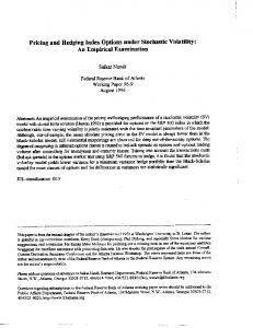
Box 2 The Volatility Skew in S&P 500 Index Options The chart illustrates the skew on four different days.1 The skew is computed from S&P 500 index options that are traded at the Chicago Board Options Exchange (CBOE). These are standard European options, for which exercise can occur only on the option expiration date, and their payoffs are determined by the level of the S&P 500 index on the option maturity date. The BlackScholes equation is used to infer the volatility using the other option formula inputs and the quoted option price. Each chart contains implied volatilities from puts and calls that were traded between 10:00 A.M. and 2:30 P.M. All options had forty-five days to maturity. Diamonds are the implied volatilities derived from individual put transactions, and squares are implied volatilities from individual call transactions. The volatilities are plotted against the ratio of the option strike to the index level. Thus, a value of one corresponds to puts or calls being at
24
Economic Review
the money. Ratios less than one represent strike prices that are out-of-the-money for puts and in-the-money for calls. The most noticeable feature of each of these plots is that the deep-out-of-the-money puts have implied volatilities substantially above the volatilities of other options. These volatilities decline almost linearly as the strike-index ratio increases. Similar smile effects have been observed in interest rate option markets (see Amin and Morton 1994 for Eurodollar futures options and Abken and Cohen 1994 for Treasury bond futures options) and in foreign exchange markets (Bates 1995). Note 1. These prices are from a CBOE data base that covers the years 1990-92. More recent smiles computed from settlement price data have the same shape as those illustrated in the charts.
December 1996
Volatility Smiles
(Options Quotes from 10:00-14:30) Puts
Calls Volatility
1/31/90
0.5
0.3
0.1 0.6
0.8
Strike/Index
1.0
1.2
1.0
1.2
1.0
1.2
1.0
1.2
1/31/91 0.5
0.3
0.1 0.6
0.8
Strike/Index 7/31/91
0.5
0.3
0.1 0.6
0.8
Strike/Index 7/31/92
0.5
0.3
0.1 0.6
Federal Reserve Bank of Atlanta
0.8
Strike/Index
Economic Review
25
The future volatility depends on a constant and a constant proportion of the last period’s volatility. In this case, the constant variance of the asset returns in the Black-Scholes formula can be replaced by the average variance that is expected to prevail from time t until time T (the expiration time), which is approximately given by 1 T 2 ∑ σu , T − t u=t
and the Black-Scholes formula can continue to be used. A more general case specifies volatility as a function of other information known to market participants. One alternative of this kind posits volatility as a function of the level of the asset price: s(S). One particular model of this type, known as the constant elasticity of variance (CEV) model, in which volatility is proportional to the level of the stock price raised to a power, appeared early in the option pricing literature (Cox and Steve Ross 1976). However, the CEV model proved not to be free of pricing biases (David Bates 1994). A more recent variation on this volatility specification was developed by Rubinstein (1994). Instead of assuming a particular form of the volatility function, Rubinstein’s method effectively infers the dependence of volatility on the level of the asset price from traded options at all available strike prices. He calls the model “implied binomial trees” because the implied risk-neutral distribution (which depends on the volatility) of the asset price at maturity is inferred from option prices by constructing a so-called binomial tree for movements of the asset price.1 (See Box 3 for a discussion of risk-neutral valuation.) Related models have been proposed by Emanuel Derman and Iraz Kani (1994), Bruno Dupire (1994), and David Shimko (1993). In a recent empirical test of deterministic-volatility models, including binomial tree approaches, Bernard Dumas, Jeffrey Fleming, and Robert Whaley (1996) show that the Black-Scholes model does a better job of predicting future option prices. The option delta, which is derived from an option pricing model and measures the sensitivity of the option price to changes in the underlying asset price, can be used to specify positions in options that offset underlying asset price movements in a portfolio. The authors demonstrate that the Black-Scholes model resulted in better hedges than those from models based on deterministic-volatility functions. For their tests based on using S&P 500 index options prices, they conclude that “simpler is better” (20). The authors note that one reason for the better 26
Economic Review
performance of the Black-Scholes model is that errors, from various sources, in quoted option prices distort parameter estimates for deterministic-volatility models and consequently degrade these models’ predictions. However, hedging performance, which is a key consideration for risk managers and traders alike, has not been systematically tested across all option pricing models. As noted below, other research indicates that some versions of stochastic-volatility models may outperform the simple Black-Scholes model in terms of hedging. ARCH Models. Autoregressive conditional heteroscedasticity (ARCH) models for volatility are a type of deterministic-volatility specification that makes use of information on past prices to update the current asset volatility and have the potential to improve on the Black-Scholes pricing biases. The term autoregressive in ARCH refers to the element of persistence in the modeled volatility, and the term conditional heteroscedasticity describes the presumed dependence of current volatility on the level of volatility realized in the past. ARCH models provide a wellestablished quantitative method for estimating and updating volatility. ARCH models were introduced by Robert F. Engle (1982) for general statistical time-series modeling. An ARCH model makes the variance that will prevail one step ahead of the current time a weighted average of past squared asset returns, instead of equally weighted squared returns, as is done typically to compute variance (see Box 1). ARCH places greater weight on more recent squared returns than on more distant squared returns; consequently, ARCH models are able to capture volatility clustering, which refers to the observed tendency of high-volatility or low-volatility periods to group together. For example, several consecutive abnormally large return shocks in the current period will immediately raise volatility and keep it elevated in succeeding periods, depending on how persistent the shocks are estimated to be. Assuming no further large shocks, the cluster of shocks will have a diminishing impact as time progresses because more distant past shocks get less weight in the determination of current volatility. Some technical features of ARCH models also make them attractive compared with many other types of option pricing models that allow for time-varying volatility. In an ARCH model, the variance is driven by a function of the same random variable that determines the evolution of the returns.2 In other words, the random source that affects the statistical behavior of returns and volatility through time is the same. December 1996
Box 3 Risk-Neutral Valuation The risk-neutral approach to option valuation was pioneered by Cox and Ross (1976) and then developed systematically by Harrison and Kreps (1979) and Harrison and Pliska (1981). It was motivated by the observation that the Black-Scholes option pricing formula does not depend on any parameters that reflect investors’ preferences toward risk—that is, their risk-return trade-offs. The key assumption is merely that investors prefer more wealth to less wealth. In particular, the option price does not depend on the expected return of the asset, which is determined by investor preferences. Since the option price does not depend on investors’ attitudes toward risk, the same option price will result irrespective of the form of investor preferences. A very convenient preference is “risk neutrality.” A risk-neutral investor cares only about the average level of wealth that can be attained by trading in a risky asset and pays no attention to the associated risk. If investors are risk-neutral, then in equilibrium the expected returns on all assets in the economy have to equal the risk-free rate; otherwise, investors would attempt to buy (sell) those securities that have expected returns greater (less) than the return on the risk-free rate, driving the expected return to equality with the risk-free rate. Therefore, under risk neutrality, the dynamics of the returns process—that is, the statistical behavior of returns through time—has to be adjusted to make the mean return on the risky asset equal to the risk-free rate. As an example, consider an asset whose returns process is described by the following equation: rt = µ + ste1,t ,
(1)
where e1,t is a random variable that is distributed normally with mean zero and variance of unity (a unit normal random variable). This equation is sometimes called the law of motion or dynamics for the return process. The mean return on the asset is µ. The realizations of the random variable e1,t make the returns rt (at time t) different from µ, and these realizations are referred to as innovations. The above equation can be rewritten using a different normal random variable v1,t, with zero mean and unit variance, rt = rft + st v1,t,,
return of the asset, equals rft . For option pricing, the law of motion of the asset returns that is relevant is (2) and not (1). Since the mean return of the asset under (2) is the risk-free rate, (2) is also known as the law of motion of the asset under the risk-neutral distribution—an environment in which all risky assets have expected returns equal to the risk-free rate. One of the key results of option pricing theory is that the price of an option, or any financial claim that has an uncertain future payoff, is given by the mathematical expectation of its payoff at its maturity, discounted at the risk-free rate. The computation of this expectation assumes that the returns of the asset follow risk-neutral dynamics, such as the example given by equation (2). If there is a second random variable that affects the price of the option, then, as in the previous example, the mean of that state variable is adjusted to give the dynamics of the state variable in a risk-neutral world. Suppose the variance s 2t follows the random process s t2 = s t2–1 + k(u – s t2–1) + gst e2,t ,
(3)
where e2,t is a standard normal random variable. The above equation is the discrete-time counterpart of the continuous-time variance process given in Heston (1993), in which the variance “reverts” to its long-term mean u at rate k, and the volatility of the variance itself is measured by g. A risk-neutralized representation of the above process analogous to (2) is s t2 = s t2–1 + k*(u* – s t2–1) + gst e*2,t.
(4)
The shock e*2,t is another standard normal random variable, and k* and u* are obtained from k and u by a riskadjustment procedure (see Heston 1993). In this case, the value of the option is equal to the mathematical expectation under the risk-neutral distribution as generated by (2) and (4), although the statistical behavior of returns and variance in the real world is generated by (1) and (3). The risk-neutral distribution itself can be inferred from traded option prices. See Abken (1995) for a basic illustration and Abken, Madan, and Ramamurtie (1996) and Aït-Sahalia and Lo (1995) for advanced approaches.
(2)
where rft is the risk-free rate. Thus, under the law of motion governed by the innovation process, v1,t, the mean
Federal Reserve Bank of Atlanta
Economic Review
27
As a result, volatility can be estimated directly from the time series of observed returns on an asset. In contrast, the direct estimation of volatility from the returns process is very difficult using stochastic-volatility models. There are many different types of ARCH models that have a wide variety of applications in macroeconomics and finance. In finance, the two most popular ARCH processes are generalized ARCH (GARCH) (Bollerslev 1986) and exponential GARCH (EGARCH) (Daniel B. Nelson 1991). The technical distinctions are beyond the scope of this article; however, researchers have tended mostly to use the GARCH process and its variations for option pricing.3 Although GARCH captures the evolution of the variance process of asset returns quite well, it turns out that there is no easily computable formula, like the Black-Scholes formula, for European option pricing under a GARCH volatility process. Instead, computer-intensive methods are used to simulate the returns and the volatility under the risk-neutral distribution in order to compute European option prices and hedge ratios. (Recent examples include Kaushik Amin and Victor Ng 1993 and Jin C. Duan 1995.) Owing to the lack of efficient pricing and hedging formulas for GARCH models, practitioners—and some researchers—often substitute the expected average variance from a GARCH model for the variance input in the Black-Scholes formula (see Engle, Alex Kane, and Jaesun Noh 1994). However, the BlackScholes formula does not hold if the variance of asset returns follows a GARCH process; such a substitution is theoretically inconsistent but may work in practice. Another problem with using the extant GARCH option pricing models is that they do not value American options, which account for most of all traded options. American options can be exercised at any time before maturity, and consequently their prices equal or exceed the prices of comparable European options by the value of this extra flexibility, termed the early-exercise premium. A simple approximation is achieved by adding an estimate of the early-exercise premium to the European price derived from a GARCH model. (There are numerical methods, such as Monte-Carlo simulations, that can value American options, but these methods are currently impractical because of the enormous number of computations required.) The value of the early-exercise premium is often evaluated using the Barone-Adesi-Whaley (1987) formula for the Black-Scholes model. An early test of a GARCH option pricing model is Engle and Chowdhury Mustafa (1992), who examined 28
Economic Review
S&P 500 index options. Their results show that the GARCH pricing model cannot account for all of the pricing biases observed in the option market. Engle, Kane, and Noh (1994) compared the trading profits resulting from a particular trading rule by using two alternatives for the variance forecasts needed for Black-Scholes: the variance forecast from a GARCH model and the variance forecast in the form of the Black-Scholes implied volatility from a previous period. As noted above, plugging a GARCH forecast into the Black-Scholes formula is ad hoc; however, in an experiment using S&P 500 index options, Engle, Kane, and Noh produced greater hypothetical trading profits using the GARCH volatility forecast than they did using the Black-Scholes implied volatility. To summarize, although GARCH is a good description of the evolution of the variance process of the asset returns, option pricing models based on GARCH are computationally demanding and may not be very useful for many practitioners given current computing technology. In addition, only a limited number of empirical tests have been done to date on GARCH option pricing models; as a consequence, it is hard to say how well the model does in pricing options and evaluating hedge ratios.4 Exponentially Weighted Moments Models. David G. Hobson and L.C.G. Rogers (1996) propose a new type of option pricing model for time-varying volatility that also has the potential to match the observed volatility smile. Their mathematical specification allows past asset-price movements to feed back into current volatility. This characteristic has some of the flavor of a GARCH model in terms of a similar feedback effect; however, the type of feedback can be much more general than encountered in standard GARCH models. Also like GARCH, but unlike standard stochastic-volatility models, there is only one source of uncertainty that drives both the asset price and its volatility.5 The Hobson-Rogers model captures past asset price volatility through a so-called offset function. The feedback relationship is primarily embodied in the functional dependence of the volatility on the offset function. The intuition behind the offset function is apparent from its form: St( m ) =
∞
∑ λe − λu ( Zt − Zt −u )m ,
u =1
St(m)
where is the value of the function at time t and m is the order of the function.6 This function simply weights deviations of a transformed current price Zt (a “discounted” logarithm of the price) from its value u December 1996
periods ago, (Zt – Zt–u), raised to the power m. The power applied to the deviation, or order of the offset function, is technically the statistical moment of the offset that is employed. For example, a first-order offset function (m = 1) considers the deviation itself, whereas a second-order offset function takes the squares of those deviations and therefore consists of a measure related to the variances of those deviations. The weighting is done by an exponential function that through the parameter l places more or less importance on the past relative to the present. A high value for l implies that recently experienced changes in the asset price have a much greater impact on volatility (and the drift) than more distant past shocks. This weighting is similar to the treatment of past return shocks in ARCH modeling. A low l gives relatively more weight to the past shocks. The persistence of past shocks l can be estimated indirectly from options prices. The feedback mechanism in this model works primarily through the asset price volatility, which can take any number of functional forms. Hobson and Rogers consider one simple form in detail in their paper. They show that even a simple version of the offset function, with m = 1, can give option prices that when substituted into the Black-Scholes equation generate a volatility smile in implied Black-Scholes volatilities evaluated at different strike prices, mimicking the smile observed in actual markets. The impact of the Hobson-Rogers assumption about the volatility specification and the persistence of volatility on option prices needs to be evaluated empirically to see how it compares with Black-Scholes or any other model. The model’s ability to trace out a smile is suggestive and may indicate the model’s potential to match actual prices well; an empirical evaluation of this model has not been performed to date.
Stochastic Volatility Stochastic volatility implies that the future level of the volatility cannot be perfectly predicted using information available today. The popularity of stochastic volatility in option pricing grew out of the fact that distributions of the asset returns exhibit fatter tails than those of the normal distribution (Benoit Mandelbrot 1963 and Eugene F. Fama 1965). In other words, the observed frequency of extreme asset returns is much higher than would occur if returns were described by a normal distribution. Stochastic-volatility models can Federal Reserve Bank of Atlanta
be consistent with fat tails of the return distribution. The occurrence of fat tails would imply, for example, that out-of-the-money options would be underpriced by the Black-Scholes model, which assumes that returns are normally distributed. However, the fat-tailed asset return distributions can also come from ARCHtype volatility as well as from jumps in the asset returns (Robert C. Merton 1976). Stochastic-volatility models could also be an alternative explanation for skewness of the return distribution. Despite the relative complexity of stochastic-volatility models, they have been popular with researchers, and additional justification for these models has recently come to light in the literature on asymmetric information about the future asset price and its impact on traded options.7 In a stochastic-volatility model, volatility is driven by a random source that is different from the random source driving the asset returns process, although the two random sources may be correlated with each other. In contrast to a deterministic-volatility model in which the investor incurs only the risk from a randomly evolving asset price, in a stochastic-volatility environment, an investor in the options market bears the additional risk of a randomly evolving volatility. In a deterministicvolatility model, an investor can hedge the risk from the asset price by trading an option and a risk-free asset based on a risk exposure computed using an option pricing formula (see Cox and Rubinstein 1985). (Equivalently, the option’s payoff can be replicated by trading the underlying asset and a risk-free asset.) However, with a random-volatility process, there are two sources of risk (the risk from the asset price and the volatility risk); a risk-free portfolio cannot be created as in the Black-Scholes model. After hedging, there is a residual risk that stems from the random nature of the volatility process. Since there is no traded asset whose payoff is a known function of the volatility, volatility risk cannot be perfectly hedged. In order to bear this volatility risk, rational investors would demand a “volatility risk” premium, which has to be factored into option prices and hedge ratios.8 A feature of stochastic-volatility models that is not shared by deterministic-volatility models is that the price of an option can change without any change in the level of the asset price. The reason is that the option price is driven by two random variables: the asset price and its volatility. In stochastic-volatility models, these two variables may not be perfectly correlated, implying that the expected volatility over the life of the option may change without any change in the asset price. The change in volatility alone can cause the option price to change. Economic Review
29
Most stochastic-volatility models assume that volatility is mean reverting. That is, although volatility varies from day to day, there is a presumed long-run level toward which volatility settles in the absence of additional shocks. Market participants refer to this feature as “regressing to the mean” of the volatility. (The evidence for this phenomenon is especially strong in markets for interest rate derivatives. See, for example, Robert Litterman, Jose Scheinkman, and Laurence Weiss 1991 and Amin and Andrew Morton 1994.) Stochastic-volatility models can be classified into two broad categories: those that lack closed-form solu-
The modeling of volatility and its dynamics is a difficult task because the path of volatility during the life of an option is highly unpredictable.
tions for European options and those that have closedform solutions.9 Even if a model’s parameters are known, most stochastic-volatility option pricing models are computationally demanding for pricing European options and especially so for pricing American options. A notable exception is the model of Steven Heston (1993) that gives closed-form solutions for prices and hedge ratios of European options. All other models compute option prices either by numerically solving a complicated partial differential equation or by Monte Carlo simulation. However, many key parameters are not readily estimated from data, particularly those of the volatility process, because, unlike the returns process of the underlying asset, the volatility process is not directly observable. Since parameter estimation is often time-consuming, the lack of readily computed solutions for option prices in many stochasticvolatility models can compound the difficulties of estimation. Although stochastic-volatility pricing models give only closed-form solutions for European options, a good approximation for the price of an American option can be obtained by adding an early exercise premium using the Barone-Adesi-Whaley approximation 30
Economic Review
in the same way as for ARCH models. Examples of this practice are in Hans J. Knoch (1992) and Bates (1995). At present, the only other way to price American options under stochastic volatility is by solving a second-order partial differential equation (Angelo Melino and Stuart Turnbull 1992), which is extremely computationally burdensome. Stochastic-Volatility Option Models without Closed-Form Solution. John C. Hull and Alan White (1987), Louis O. Scott (1987), and James B. Wiggins (1987) were among the first to develop option pricing models based on stochastic volatility. Hull and White as well as Scott made the questionable assumption that the risk premium of volatility is zero—that is, the volatility risk is not priced in the options market—and that volatility is uncorrelated with the returns of the underlying asset. Wiggins, who also assumed a zero-volatility risk premium, found that the estimated option values under stochastic volatility were not significantly different from Black-Scholes values, except for long maturity options. For equity options, Christopher Lamoureux and William Lastarapes (1993) offer evidence against the assumption of a zero-volatility risk premium. For currency options, Melino and Turnbull (1992) found that a random-volatility model yields option prices that are in closer agreement with the observed option prices than those of the Black-Scholes model. While the numerical methods and computers currently available allow computation of these stochasticvolatility option prices, they are still largely impractical for determining hedge ratios, which are vital to marketmakers, dealers, and others. As a result, these stochastic-volatility models may not currently be useful for practitioners. Nevertheless, development of stochasticvolatility models continues as researchers attempt to find more tractable models. Stochastic-Volatility Models with Closed-Form Solutions. Elias M. Stein and Jeremy C. Stein (1991) develop a European option pricing model under stochastic volatility that is somewhat easier to evaluate than the models described above. 10 Although less computationally expensive than the other models, the authors make the unrealistic assumption of zero correlation between the volatility process and the returns of the underlying asset. Heston (1993) was the first to develop a stochasticvolatility option pricing model for European equity and currency options that can be easily implemented, is computationally inexpensive, and allows for any arbitrary correlation between asset returns and volatility.11 The model gives closed-form solutions not only for option prices but also for the hedge ratios like the December 1996
deltas and the vegas of options. (Delta and vega measure the sensitivity of the option price to changes in the asset price and to changes in the volatility, respectively. Knowledge of these measures enables the construction of hedges for options or for portfolios containing embedded options.) In this model, the asset returns rt and the variance st2 are assumed to evolve through time as rt = µ + ste1,t and 2 2 + k(u – st–1 ) + gste2,t, st2 = st–1
respectively, where e1,t and e2,t are two standard normal random variables that could be correlated with each another, either positively or negatively, with a correlation coefficient, r. Equivalently, this coefficient also measures the correlation between the return of the asset and the volatility process. In this model, the variance evolves through time in such a way that its long-run average level is measured by u and the speed with which it is pulled toward this long-run mean is measured by k, also known as the mean-reversion coefficient. The variable g is a measure of the volatility of variance. If g is zero, the model simplifies to a time-varying deterministic-volatility model. In the finance literature, this process for the volatility is also known as a square-root volatility process. The particular nature of the process ensures that volatility “reflects” away from zero: if volatility ever becomes zero, then the nonzero k ensures that volatility will become positive. Note that st2 in this model is not directly comparable to the implied variance from the Black-Scholes model. The reason is that s2t represents the instantaneous variance (at time t), whereas the implied variance in the Black-Scholes model is the average expected variance through the life of an option and need not equal the instantaneous variance if the model is not true. In Heston’s model, the average expected variance during the life of an option is a function of the instantaneous variance, the long-run average variance, the speed with which the instantaneous variance adjusts, and the time to expiration of the option. The option price and hedge ratios in Heston’s model are functions not only of the parameters that appear in the Black-Scholes formula but also of k, u, r, g, and an additional parameter, l. The parameter l is a constant such that ls2t measures the risk premium of volatility. The volatility risk premium is assumed to be Federal Reserve Bank of Atlanta
directly proportional to the level of the volatility. The need for an assumption about the form of the volatilityrisk premium is a weakness of any stochastic-volatility model because the form of the volatility-risk premium cannot be deduced from the weak assumption that all investors prefer more wealth to less wealth, as discussed in Box 3, but requires assumptions on investor tolerance toward risk that in general are difficult to justify. In this model, the form of the volatility-risk premium is crucial because it enables the derivation of the closed-form solutions for option prices and hedge ratios. However, it should not be interpreted as a weakness of this model vis-à-vis other stochasticvolatility models of option prices because others make the even stronger and less plausible assumption that the risk premium of volatility is zero. The parameters r and g are very important for determining the form of the risk-neutral distribution of the asset price at the time of the option’s expiration (the terminal asset price) and hence the current option price. In other words, they may be important for accounting for the smile effects seen in the chart. For example, consider the probability that a European call option will finish in the money. Ceteris paribus, an increase in g (an increase in the volatility of volatility) makes the tails of the risk-neutral distribution fatter: the occurrence of extreme returns is more likely.12 The sign and magnitude of r determines the sign and extent of skewness in the risk-neutral distribution of the terminal asset price. Positive correlation implies that an increase in the returns of the underlying asset is associated with an increase in the volatility, tending to make the right tail of the distribution thicker and the left tail thinner than those of a normal distribution of asset returns. In other words, the frequency of extreme positive outcomes is higher and the frequency of extreme negative outcomes is lower than in the BlackScholes model—that is, the returns have positive skewness. As a result, prices of out-of-the-money calls, which benefit from this scenario of positive skewness, are higher in the stochastic-volatility model than corresponding Black-Scholes call prices, and those of out-of-the-money puts (that lose under this scenario) are lower. On the other hand, a negative correlation implies that a decrease in the returns of the underlying asset is associated with an increase in the variance. Therefore, the left tail would be thicker and the right tail thinner than assumed for the Black-Scholes model. Since out-of-the-money puts benefit from a thicker left tail, market prices for these options would be higher than in the Black-Scholes model (underpricing by the Black-Scholes model), and, similarly, out-of-the-money Economic Review
31
calls that lose from a thicker left tail would be overpriced by the Black-Scholes model. This last scenario is consistent with observations in the market for S&P 500 index options since the crash of 1987. As noted earlier, out-of-the-money puts have tended to command much higher prices than can be explained by the Black-Scholes model, whereas out-ofthe-money calls are overpriced by the Black-Scholes model. According to the stochastic-volatility model, the underpricing of the out-of-the-money puts and overpricing of out-of-the-money calls by the BlackScholes model—the volatility skew—could be the result of a negative correlation between index returns and a random volatility process.
A likely cause of financial market volatility is the arrival of information and its subsequent incorporation into asset prices through trading.
The empirical work done on Heston’s model includes that by Knoch (1992), Saikat Nandi (1996), and Bates (1995). In order to take into account the possibility of sudden large price movements, such as the crash of 1987, Bates generalizes Heston’s model by allowing for jumps in asset prices. While Knoch and Bates study the pricing issues of this model for options on foreign currencies, Nandi examines both pricing and hedging issues using the S&P 500 index options. All of these studies find that Heston’s model is able to generate prices that are in closer agreement with market option prices than those of the Black-Scholes model. However, it is not the case that this model is able to explain all biases of the Black-Scholes model. While it is true that the remaining pricing biases are of smaller magnitude than those of the Black-Scholes model, Nandi finds that there are still substantial biases for out-of-the-money puts and calls in the S&P 500 index options market. In particular, the model underprices out-of-the-money puts and overprices out-of-the-money calls. It is possible that the square-root volatility process and therefore the model itself are misspecified. 32
Economic Review
This misspecification would be unfortunate because the particular form of the volatility process is what makes this stochastic-volatility model tractable. If the Black-Scholes assumption of constant volatility were true, a hedge portfolio (hedged against the risk from the asset price) would simply earn the riskfree rate of return. Such a portfolio would typically consist of a position in the underlying asset and an option. The position would be altered through time by trading, based on the formulas for hedge ratios determined by the Black-Scholes model (see Cox and Rubinstein 1985) or other option pricing models. When volatility is stochastic, as it probably is in the real world, hedging using the Black-Scholes model does not result in risk-free positions. A stochastic-volatility model may do a better job of hedging against price and volatility risks. Nandi (1996) finds that for S&P 500 index options the returns of a hedge portfolio constructed using Heston’s stochastic-volatility model come closer to matching a risk-free return through time better than hedge portfolio returns obtained using the Black-Scholes model. Volatility Jumps. All the time-varying volatility models that have been discussed so far assume that the volatility of the underlying asset as well as its price evolves “smoothly,” though randomly, through time: there are no jumps in the volatility process. However, a likely cause of financial market volatility is the arrival of information and its subsequent incorporation into asset prices through trading. To the extent that information—“news”—arrives in discrete lumps, it is possible that volatility shifts between episodes of low and high volatility. For example, uncertainty about an impending news release (concerning some macroeconomic variable, like an anticipated change in the fed funds rate by the Federal Open Market Committee) may cause the volatility of an asset price to rise. However, after a few rounds of trading, with the information having been incorporated into asset prices, volatility may revert back to its previous level. To account for jumps like those in the example, Vasantlilak Naik (1993) develops a pricing model for European options in which volatility switches between low and high levels. Each level or “regime” is expected to last for a certain period of time that is not known a priori. One tractable version of his model assumes that the risk from the volatility jumps is not priced by market participants. The model takes the same parameters that enter the Black-Scholes formula as well as additional parameters such as the probabilities of jumps from one regime to another regime, given that volatility is currently in a particular regime. Naik finds December 1996
that short-maturity options are much more sensitive to volatility shifts than long-maturity options. The reason is that, over a long period of time, expected upward and downward jumps in volatility are canceled by each other, resulting in a volatility that is close to the normal level. This model has not been empirically tested and therefore cannot yet be evaluated against other stochasticvolatility models. In general, jump models can be difficult to verify empirically because jumps occur infrequently. The parameters of such models may be imprecisely estimated using relatively small historical data series on option prices or underlying asset prices.
Conclusion Since volatility of the underlying asset price is a critical factor affecting option prices, the modeling of volatility and its dynamics is of vital interest to traders, investors, and risk managers. This modeling is a difficult task because the path of volatility during the life of an option is highly unpredictable. Clearly, the BlackScholes assumption of constant volatility can be improved upon by incorporating time variation in volatility.
While deterministic-volatility models can capture the dynamics of the volatility reasonably well, many of these option pricing models, such as ARCH models, are computationally expensive, especially for American options. Deterministic-volatility option pricing models have the advantage that most parameters can be estimated directly from the observable time series of returns data. However, superior hedging performance of such models relative to that of the Black-Scholes model has not been demonstrated. On the other hand, there is evidence that some stochastic-volatility option pricing models provide better hedges than BlackScholes, although for stochastic-volatility option pricing models and volatility-jump models, parameter estimation is typically demanding and problematic. The development of tractable stochastic-volatility models as well as more efficient methods of model parameter estimation are currently an area of intensive research. For both academic researchers and market practitioners, no consensus exists regarding the best specification of volatility for option pricing. Although a number of alternative approaches can account, at least partially, for the pricing deficiencies of the Black-Scholes model, none dominates as a clearly superior approach for pricing options.
Notes 1. Instead of taking a wide range of values as in the real world, a binomial tree restricts stock price movements at any moment in time to be either up with one probability or down with another (see Cox and Rubinstein 1985). 2. Although there is one source of uncertainty that drives both the asset returns and the volatility in a GARCH model, which is a special case of ARCH, the asset returns are distributed continuously—that is, one out of an infinite number of possible uncertain returns will be realized over the next period. Therefore, with discrete trading (as in a GARCH model), it is not possible to replicate all possible uncertain returns outcomes (see Duffie and Huang 1985) by trading in the option and a risk-free asset (or, equivalently, a unique risk-free portfolio cannot be created by trading in the underlying asset and an option). Hence, a risk premium associated with the returns of the underlying asset is required in a GARCH model. 3. The NGARCH of Engle and Ng (1993) is one such variation. 4. GARCH can capture the volatility smile. In a GARCH model, such as Duan’s (1995), the price of an option, besides being a function of the variables that appear in the
Federal Reserve Bank of Atlanta
Black-Scholes formula, is also a function of variables that describe the time variation in volatility as well as a variable that accounts for the risk premium of the asset returns, that is, the excess return over a risk-free asset. Since the risk premium summarizes investor preferences, the GARCH option pricing model is not preference-free—a key attribute of the Black-Scholes model. Duan shows that under the riskneutral distribution, the value of the GARCH variance at a point in time is negatively correlated with past asset returns if the risk premium of the asset is greater than zero. Such a negative correlation can give rise to negative skewness in the risk-neutral distribution, which seems to be a feature of the empirical data, as discussed in Bates (1995). GARCH models can therefore potentially generate option prices that are consistent with the observed volatility skew. 5. The Hobson-Rogers model is also preference-free. This model, unlike GARCH, is set in continuous time. There being a single source of uncertainty and continuous trading, all possible uncertain returns outcomes of the underlying risky asset over the next period can be replicated by trading in an option and a risk-free asset (Duffie and Huang 1985), and there is no need for any risk premium of returns.
Economic Review
33
6. The Hobson-Rogers equation actually is written with an integral rather than a summation. 7. Back (1993) shows how stochastic volatility might be introduced endogenously in asset markets due to asymmetric information about the future price of an underlying asset on which an option is traded. 8. In an ARCH option pricing model the risk premium that enters is the risk premium of asset returns and not the risk premium of volatility. 9. For American options, a closed-form solution in a stochasticvolatility model has not yet been derived. 10. Their model requires the numerical evaluation of a twodimensional integral (that is computationally easier) rather
than the solution of a second-order partial differential equation. However, the volatility process is allowed to become negative, an undesirable feature. 11. Heston’s (1993) paper gives the closed-form solution for prices of call options. The price of a put option can be easily obtained using the put-call parity for European options. 12. A tail of a probability distribution is the area under the distribution that assigns probabilities to extreme outcomes. For example, in the typical bell-shaped normal distribution, there are two tails, the right tail and the left tail, that slowly taper off.
References Abken, Peter A. “Over-the-Counter Financial Derivatives: Risky Business?” Federal Reserve Bank of Atlanta Economic Review 79 (March/April 1994): 1-22. ——. “Using Eurodollar Futures Options: Gauging the Market’s View of Interest Rate Movements.” Federal Reserve Bank of Atlanta Economic Review 80 (March/April 1995): 10-30. Abken, Peter A., and Hugh Cohen. “Generalized Method of Moments Estimation of Heath-Jarrow-Morton Models of Interest-Rate Contingent Claims.” Federal Reserve Bank of Atlanta Working Paper 94-8, August 1994. Abken, Peter A., Dilip B. Madan, and Sailesh Ramamurtie. “Estimation of Risk-Neutral and Statistical Densities by Hermite Polynomial Approximation: With an Application to Eurodollar Futures Options.” Federal Reserve Bank of Atlanta Working Paper 96-5, June 1996. Aït-Sahalia, Yacine, and Andrew W. Lo. “Nonparametric Estimation of State-Price Densities Implicit in Financial Asset Prices.” National Bureau of Economic Research Working Paper 5351, 1995. Amin, Kaushik, and Andrew Morton. “Implied Volatility Functions in Arbitrage-Free Term Structure Models.” Journal of Financial Economics 35 (1994): 141-80. Amin, Kaushik, and Victor Ng. “ARCH Processes and Option Valuation.” University of Michigan Working Paper, 1993. Back, Kerry E. “Asymmetric Information and Options.” Review of Financial Studies 6 (1993): 435-72. Barone-Adesi, Giovanni, and Robert Whaley. “Efficient Analytic Approximation of American Option Values.” Journal of Finance 42 (1987): 301-20. Bates, David. “The Skewness Premium: Option Pricing under Asymmeric Processes.” University of Pennsylvania Working Paper, 1994. ——. “Jumps and Stochastic Volatility: Exchange Rate Processes Implicit in Deutschemark Options.” Review of Financial Studies 9 (1995): 69-107. Black, Fischer, and Myron S. Scholes. “The Pricing of Options and Corporate Liabilities.” Journal of Political Economy 81 (May/June 1973): 637-54.
34
Economic Review
Bollerslev, Tim. “Generalized Autoregressive Conditional Heteroscedasticity.” Journal of Econometrics 31 (1986): 30727. Bollerslev, Tim, Ray Y. Chou, and Kenneth F. Kroner. “ARCH Modeling in finance: A Review of the Theory and Empirical Evidence.” Journal of Econometrics 5 (1992): 5-59. Cox, John C., and Steve Ross. “The Valuation of Options for Alternative Stochastic Processes.” Journal of Financial Economics 3 (1976): 145-66. Cox, John C., and Mark Rubinstein. Options Markets. Englewood Cliffs, N.J.: Prentice Hall, 1985. Derman, Emanuel, and Iraz Kani. “Riding on the Smile.” Risk 7 (February 1994): 32-39. Duan, Jin C. “The GARCH Option Pricing Model.” Mathematical Finance 5 (1995): 13-32. Duffie, Darrell, and Chi-Fu Huang. “Implementing ArrowDebreu Equilibria by Continuous Trading of Few LongLived Securities.” Econometrica 53, no. 6 (1985): 1337-56. Dumas, Bernard, Jeffrey Fleming, and Robert Whaley. “Implied Volatility Functions: Empirical Tests.” Rice University Working Paper, 1996. Dupire, Bruno. “Pricing with a Smile.” Risk 7 (January 1994): 18-20. Engle, Robert F. “Autoregressive Conditional Heteroscedasticity with Estimates of the Variance of U.K. Inflation.” Econometrica 50 (1982): 987-1008. Engle, Robert, Alex Kane, and Jaesun Noh. “Forecasting Volatility and Option Prices of the S&P 500 Index.” Journal of Derivatives (1994): 17-30. Engle, Robert F., and Chowdhury Mustafa. “Implied ARCH Models from Option Prices.” Journal of Econometrics 52 (1992): 289-311. Engle, Robert, and Victor Ng. “Measuring and Testing the Impact of News on Volatility.” Journal of Finance 48 (1993): 1749-78. Fama, Eugene F. “The Behavior of Stock Market Prices.” Journal of Business 38 (1965): 34-105.
December 1996
Harrison, J. Michael, and David Kreps. “Martingales and Arbitrage in Multiperiod Securities Markets.” Journal of Economic Theory 20 (1979): 381-408. Harrison, J. Michael, and Stanley Pliska. “Martingales and Stochastic Integrals in the Theory of Continuous Trading.” Stochastic Processes and Their Applications 11 (1981): 215-60. Heston, Steven. “A Closed-Form Solution for Options with Stochastic Volatility with Applications to Bond and Currency Options.” Review of Financial Studies 6 (1993): 327-43. Hobson, David G., and L.C.G. Rogers. “Complete Models with Stochastic Volatility.” University of Bath, School of Mathematical Sciences. Unpublished paper, 1996. Hull, John C., and Alan White. “The Pricing of Options on Assets with Stochastic Volatilities.” Journal of Finance 42 (1987): 281-300. Knoch, Hans J. “The Pricing of Foreign Currency Options with Stochastic Volatility.” Ph.D. dissertation, Yale School of Organization and Management, 1992. Lamoureux, Christopher, and William Lastarapes. “Forecasting Stock-Return Variance: Toward an Understanding of Stochastic Implied Volatilities.” Review of Financial Studies 6 (1993): 293-326. Litterman, Robert, Jose Scheinkman, and Laurence Weiss. “Volatility and the Yield Curve.” Journal of Fixed Income Research (June 1991): 49-53. Mandelbrot, Benoit. “The Variation of Certain Speculative Prices.” Journal of Business 36 (1963): 394-419. Melino, Angelo, and Stuart Turnbull. “The Pricing of Foreign Currency Options with Stochastic Volatility.” Journal of Econometrics 45 (1992): 239-65.
Federal Reserve Bank of Atlanta
Merton, Robert C. “Option Pricing with Discontinuous Returns.” Journal of Financial Economics 3 (1976): 125-44. Naik, Vasantlilak. “Option Valuation and Hedging Strategies with Jumps in the Volatility of Asset Returns.” Journal of Finance 48 (1993): 1969-84. Nandi, Saikat. “Pricing and Hedging Index Options under Stochastic Volatility: An Empirical Examination.” Federal Reserve Bank of Atlanta Working Paper 96-9, August 1996. Nelson, Daniel B. “Conditional Heteroscedasticity in Asset Returns: A New Approach.” Econometrica 59 (1991): 347-70. Rubinstein, Mark. “Nonparametric Tests of Alternative Option Pricing Models Using All Reported Trades and Quotes on the 30 Most Active Option Classes from August 23, 1976, through August 31, 1978.” Journal of Finance 40 (1985): 455-80. ——. “Implied Binomial Trees.” Journal of Finance 49 (1994): 771-818. Scott, Louis O. “Option Pricing When the Variance Changes Randomly: Theory, Estimation, and Application.” Journal of Financial and Quantitative Analysis 22 (1987): 419-38. Shimko, David. “Bounds on Probability.” Risk 6 (April 1993): 33-37. Stein, Elias M., and Jeremy C. Stein. “Stock Price Distributions with Stochastic Volatility: An Analytic Approach.” Review of Financial Studies 4 (1991): 727-52. Wiggins, James B. “Option Values under Stochastic Volatilities.” Journal of Financial Economics 19 (1987): 351-72.
Economic Review
35