How a Dummy Replaces a Student’s Test and Gets an F (Or, How Regression Substitutes for t tests and ANOVA) OTeaching riginal UK Articles 28 Blackwell Oxford, Teaching ·TEST 20141-982X Statistics Publishing Statistics. Volume Ltd 28, Number 2, Spring 2006
Joseph G. Eisenhauer
KEYWORDS: Teaching; Regression; Dummy variables; Analysis of variance; t tests.
Canisius College, Buffalo, New York, USA e-mail:
[email protected] Summary Using dummy variables, this note offers a convenient illustration to demonstrate that regression can replace both the one-factor analysis of variance and the two-population t test with independent random samples. The exercise also helps to develop students’ intuition regarding regression coefficients.
ª INTRODUCTION ª ost statistics text-books rightly introduce the one-factor analysis of variance (ANOVA) as an extension or generalization of the t test for comparing two population means using independent random samples. The very next topic presented after ANOVA is usually regression, and many texts carefully describe the construction of an ANOVA table from regression residuals, properly interpreting the F statistic as indicating whether any of the independent variables are significant. Unfortunately, because the examples and data sets used in regression are generally quite different from those used in the previous hypothesis tests, it is natural for students to think of these as separate procedures with entirely different, almost opposite, purposes: analysis of variance for testing whether the mean of a single variable differs across several populations, and regression for finding a relationship among several different variables that characterize a single population. The notion that regression can serve as a generalization of the onefactor ANOVA and therefore as a substitute for the two-sample t test of means is almost never stated explicitly. As a consequence, an opportunity to thoroughly explore the nature and interchangeability of these procedures is often overlooked.
synthesis after all three procedures have been studied.
M
I suggest the following simple exercise, based on indicator or dummy variables, to demonstrate the linkages from t tests to F tests to regression. It may be used either to introduce regression, or as a 78
• Teaching Statistics.
Volume 28, Number 3, Autumn 2006
ª ILLUSTRATION ª Suppose we wish to test the equality of two population means with independent random samples; the null hypothesis is H0 : µ1 = µ2 and the alternative is Ha : µ1 ≠ µ2. For context, let us consider the ages of movies shown on two different television channels, as suggested by Alan Graham (1994). Perusing the Guardian Guide of 9 October 1993, Graham provides data on the years in which films shown on various TV stations during a Saturday were produced. For present purposes, I have converted those data into the age (in years) of each film, calculated as 1993 minus the year in which the film debuted. Following Graham, ‘Terrestrial’ refers to a composite of four non-satellite stations. Satellite: Terrestrial:
27 24 15 16 2 6 1 2 9 19 43 50 30 10 34 62
3
2
Note that using samples of different sizes such as those above provides a helpful hint to students that the samples are independent and not matched pairs. It should also be noted that the tests conducted below require the data to be treated as random samples taken from Normally distributed populations having equal variances. These are strong and perhaps unrealistic assumptions in the current context but, as the present purpose is merely illustrative, the plausibility of the example is not © 2006 The Author Journal compilation © 2006 Teaching Statistics Trust
Source Treatment Error Total
Sum of squares Degrees of Mean square freedom 2215.136 3418.475 5633.611
1 16 17
2215.14 213.65
F 10.368
Table 1. Analysis of variance for two TV channels
the intercept is correctly identified as 9.8 and the slope is found to be (32.125 − 9.8)/(1 − 0) = 22.325; both can thus be obtained easily, without applying calculus to minimize the sum of squared errors and thereby derive the normal equations. Second, the diagram suggests visually that both the intercept and the slope of the regression line are stochastic, sample-sensitive variables that have standard deviations associated with them. Regression software can then be used to verify that the resulting equation is indeed Age = 9.800 + 22.325 TerrTV (4.62) (6.93)
Fig. 1. Scatterplot of Age versus TerrTV
of central importance; indeed, any alternative data sets suitable for use with t tests and F tests should be sufficient for the following demonstration. After studying t tests, students should be able to calculate (either manually or by computer) the two sample means (9.8 and 32.125 years, respectively), the pooled variance ( s 2p = 213.65), and Student’s t statistic (t = 3.22), and then use the latter to reject the null hypothesis – i.e. to determine that there exists a statistically significant difference between the means. Similarly, after having learned analysis of variance, students ought to be able to construct the ANOVA in table 1 and come to the same conclusion, recognizing that the mean square due to error (MSE = 213.65) is identically equal to the pooled sample variance calculated above, while the F ratio (F = 10.368) is just the square of Student’s t. Now, to demonstrate that regression is a further generalization of the same procedure, the two samples can be combined into a single sample of 18 films. The ages of the movies represent observations of the dependent variable, and an independent dummy variable (x = TerrTV ) can be created to take the value 0 for films on satellite stations and 1 for films on terrestrial TV. In the scatter diagram for this simple linear regression, all the observations will of course have x-coordinates of either zero or one, as shown in figure 1. However, even this peculiarity provides some valuable insights. First, students generally have no difficulty surmising that a straight line should connect the means of the two clusters, which have already been calculated above as 9.8 and 32.125 years, respectively. Thus, © 2006 The Author Journal compilation © 2006 Teaching Statistics Trust
where standard errors are in parentheses. The equation confirms that when TerrTV takes the value zero (a film is played on satellite TV ), the film’s predicted age is 9.8 years; for a film shown on terrestrial television (TerrTV = 1), the predicted age increases by 22.325 years. Indeed, the t statistic for TerrTV ( t = 3.22) is identical to that produced earlier by the two-sample t test; because terrestrial and satellite stations run films of significantly different average ages, TerrTV is a significant predictor of Age. (As an interesting aside, dividing the variance of the intercept by the variance of the slope yields Σ x2/n = 8/18, the proportion of films on terrestrial TV.) And because the sum of squares due to regression is the sum of squares due to treatment, one gets exactly the same ANOVA as shown in table 1 (from which se = MSE = 14.6 and R2 = 0.393 can be found). Thus, it becomes evident that regression with a dummy variable can be used in place of the two-sample t test, as well as the F test from the one-factor ANOVA.
ª EXTENSION ª This illustration can readily be extended to multiple linear regression by including the ages of films played on a third station during the same day of the week. Graham (1994) provides production years for 11 films shown on the Movie channel, which yield the following ages. Movie:
(It is poses from equal
10
3
29
24
3
2
2
2
2
11
3
worth reiterating that for illustrative purthe data are treated as a random sample a Normal population having a variance to those of the Satellite and Terrestrial
Teaching Statistics.
Volume 28, Number 3, Autumn 2006 •
79
Source Treatment Error Total
Sum of squares Degrees of Mean square freedom 3110.171 4346.657 7456.828
2 26 28
1555.085 167.179
F 9.302
Table 2. Analysis of variance for three channels
populations.) Beginning again with t tests, students can easily determine that the average age on this channel (8.273 years) is significantly lower than the average on terrestrial stations (t = −3.6), but not significantly lower than the average on satellite stations (t = −0.36). Of course, this requires several separate comparisons of two stations at a time, and it becomes clear that comparing many means would require numerous t tests, a rather tedious prospect. Alternatively, by applying analysis of variance students can construct table 2 and, comparing the F ratio (F = 9.302) to either its 5% or 1% critical value (3.37 or 5.53, respectively), determine that at least one mean age is significantly different from another. Next, by including the additional 11 observations in the regression sample and creating a second dummy variable, MovieTV, that takes the value 1 if the film is played on the Movie channel and 0 otherwise, a multiple linear regression that encompasses the prior tests can also be performed. Age is again the dependent variable, and the two dummies, TerrTV and MovieTV, are the only independent variables. At this stage, despite the absence of a scatter diagram, alert pupils who have grasped the relationships discussed above should be able to guess what the resulting regression equation will be simply by using their intuition, and use table 2 to predict the value of R2. Their insights can then be verified by using statistical software to obtain Age = 9.80 + 22.325 TerrTV − 1.527 MovieTV (4.09) (6.13) (5.65) Just as before, the constant reflects the average age of films on satellite TV (the base case for both dummies), and the coefficient of TerrTV reveals that the films shown on terrestrial TV are, on average, 22.325 years older than those on satellite. Likewise, the coefficient of MovieTV indicates that the average film shown on the Movie channel is 1.527 years newer than the average film on satellite TV, while its t statistic (t = −0.27) indicates that this difference is not significant. Comparing the simple and multiple regression results, it may be useful to note that the inclusion of the second 80
• Teaching Statistics.
Volume 28, Number 3, Autumn 2006
dummy variable has not altered the coefficient of the first – which suggests that there is little or no multicollinearity between the two (and more formally, statistics such as variance inflation factors can easily verify this). One might even discuss the ‘dummy variable trap’ that would result from adding a third dummy. Of course, the regression package will also confirm that R2 = 0.417 and R2 = 0.372, as anticipated by the ANOVA in table 2. Naturally, other and possibly better examples can be devised to illustrate the same concepts. One limitation of the present example is that, while television stations obviously select recent or vintage films (although age is probably not their primary screening criterion), causality could be made clearer by different examples. If, for instance, similar data were interpreted as the production levels of three different machines, then the causality from the independent variables to the dependent variable would be unambiguous. Then again, one may prefer to use the movie example above as a springboard to discuss the difference between correlation and causation.
ª CONCLUSION ª Indicator variables are generally presented as a special topic in multiple linear regression, and are therefore taught near the end of a first-year university course in statistics. By that time, twosample t tests and perhaps even one-factor ANOVAs may be relatively dim memories. The exercise outlined here employs regression dummies to test for differences in means – a method that not only reinforces the earlier concepts, but also conveniently integrates several topics from various segments of the course, and thereby emphasizes their complementarities. As an additional benefit, this approach allows students to apply and develop their intuition regarding regression equations, so that the coefficients and related statistics are not quite so mysterious. Acknowledgement I thank the editor and anonymous referees for helpful comments. Any errors are my own. Reference Graham, A. (1994). Don’t discard last week’s TV guide! Teaching Statistics, 16(3), 66 – 69. © 2006 The Author Journal compilation © 2006 Teaching Statistics Trust