Jun 16, 2007 - arXiv:0706.2435v1 [gr-qc] 16 Jun 2007. Orbital Dynamics of Binary Boson Star Systems. C. Palenzuela1, L. Lehner1, S. L. Liebling2.
Orbital Dynamics of Binary Boson Star Systems C. Palenzuela1, L. Lehner1 , S. L. Liebling2 1
arXiv:0706.2435v1 [gr-qc] 16 Jun 2007
2
Department of Physics and Astronomy, Louisiana State University, 202 Nicholson Hall, Baton Rouge, Louisiana 70803-4001, USA Department of Physics, Long Island University, Brookville, New York 11548, USA
We extend our previous studies of head-on collisions of boson stars by considering orbiting binary boson stars. We concentrate on equal mass binaries and study the dynamical behavior of boson/boson and boson/antiboson pairs. We examine the gravitational wave output of these binaries and compare with other compact binaries. Such a comparison lets us probe the apparent simplicity observed in gravitational waves produced by black hole binary systems. In our system of interest however, there is an additional internal freedom which plays a significant role in the system’s dynamics, namely the phase of each star. Our evolutions show rather simple behavior at early times, but large differences occur at late times for the various initial configurations. I.
INTRODUCTION
Boson stars are compact solutions to Einstein’s gravitational field equations coupled to a massive, complex scalar field. In addition to their interest as soliton-like solutions akin to so-called Q-balls [1], they also serve as a simplified model of an astrophysical compact object with which to probe non-linear regimes. In a recent work, we described an implementation of the Einstein equations that can evolve, among other possible sources, boson star configurations [2]. We studied the head-on collision of boson stars with equal mass but possibly differing in phase and oscillation frequencies. The simulations revealed interesting effects arising from these possible differences. In particular, by adopting phase and frequency reflections the collisions displayed markedly different behavior, from merger to repulsion. In the present work we revisit these binaries in scenarios with non-vanishing angular momentum. Our interest in the present work is twofold. On the one hand, we want to understand the dynamics of the more complex scenario of orbiting stars. The presence of angular momentum in this case gives rise to richer phenomenology arising due to the orbiting behavior of the system and the peculiarities of single boson stars with angular momentum. As illustrated by stationary, axisymmetric, rotating boson star solutions whose angular momentum is quantized [3], rotating boson stars have angular momentum further constrained than their regular fluid counterparts. On the other hand, the system also probes the dynamics of compact objects in general relativity. In this context it is particularly interesting to analyze to what extent rather simple analysis can shed light on the orbiting behavior and gravitational wave output of the system. We recall that binary black hole simulations have revealed, among other features, that the dynamics and consequent radiation from binary black holes can be reasonably well approximated by perturbative approaches well beyond the limited range of validity initially assumed [4, 5]. Such a result indicates that for binary black holes, the system undergoes a rather smooth transi-
tion from a quasi-adiabatic inspiral regime to the merger and ring-down without significant nonlinearities becoming major factors. This rather simple behavior seems to be a consequence of the final object being another black hole. When this black hole forms, it encircles a larger region which ‘cuts-away’ portions of the spacetime with strong curvature and dynamics and the spacetime is described by a perturbed black hole. The binary boson stars considered in this work enable us to further examine compact binary systems in a different but certainly related context. For binary boson star cases, as for binary neutron star cases, the evolution at early stages demonstrates simple quasi-adiabatic behavior. However, as the stars approach each other, effects related to the stars’ internal structure play a significant role. Here we study binary boson stars, analyze their dynamical behavior and extract the gravitational wave output for different cases. As we discuss, significant differences arise from two effects. One effect is the same as that discussed in the headon case arising from the effective interaction energy inducing significantly different gravitational potential wells when the stars come close to each other. The other effect concerns the possible end states of the merger given the presence of angular momentum. If the merger is to produce a single remnant star, presumably it would yield, asymptotically, a stationary, spinning boson star. However, for the system to settle into one of the spinning boson stars found in [3], it would have to shed angular momentum and/or energy to be consistent with one of the quantized states. There are several “channels” for the system to achieve this. One is through radiation of angular momentum and energy; this, however, might require long dynamical times for the system to shed enough. In related orbiting systems, like binary black holes, only a few percent of the initial mass/angular momentum [6, 7, 8, 9] is radiated. Thus, extraction of energy/angular momentum via gravitational waves from the merged object is likely a small effect here as well. Other channels, such as the break-up of the merged star and black hole formation, will play significant roles in the dynamics of the system as we illustrate in this work. For a particular configuration (i.e, masses and sepa-
2 ration of the stars), the evolution of boson/boson pair appears to be highly dependent on the value of the initial angular momentum Jz . This outcome contrasts with the results of our previous work [2] which demonstrated that the (unboosted) head-on collision (Jz = 0) results in a remnant black hole when the individual masses are large. The paper is organized as follows. In Section II we briefly summarize the formalism for the Einstein-KleinGordon system, referring the reader to previous work for more details [2]. Section III describes the procedure for setting the initial data. Section IV recalls some of the analysis quantities that are going to be used along this paper. Section V describes the numerical implementation of the governing equations and the presentation of our results. We conclude in Section VI with some final comments. II.
THE EINSTEIN-KLEIN-GORDON SYSTEM
As described in [2], the dynamics of a massive complex scalar field in a curved spacetime is described by the following Lagrangian density (in geometrical units G = c = 1) [10] �i � 1 h ab ¯ 1 2 . (1) g ∂a φ∂b φ + V |φ| R+ L=− 16π 2
Here R is the Ricci scalar, gab is the spacetime metric, φ is the scalar field, φ¯ its complex conjugate, and V (|φ|2 ) = m2 |φ|2 the interaction potential with m the mass of the bosonic particle which has inverse length units. Throughout this paper Roman letters at the beginning of the alphabet a, b, c, .. denote spacetime indices ranging from 0 to 3, while letters near the middle i, j, k, .. range from 1 to 3, denoting spatial indices. This Lagrangian gives rise to the equations determining the evolution of the metric (Einstein equations) and those governing the scalar field behavior (Klein-Gordon Equations). We employ the same implementation described in [2] to simulate our systems of interest, and the reader is referred to that paper for the complete details. The only difference is with the initial data described in the following section. III.
INITIAL DATA
We adopt a simple prescription to define the initial data describing two boson stars. Throughout this work this data will be obtained by a superposition of two stars with linear momentum. In order to define such data, we adopt the spacetime and the scalar field described in [2] and boost each star either with a Galilean or Lorentz boost. While this data satisfy the constraints only approximately, the constraint violation measured on the initial data is at or below the truncation error. Furthermore, although the runs presented here have been
obtained with the Galilean boost, similar behaviour is obtained when employing a Lorentzian one, since after some transient epoch the dynamics of the system is, for the most part, insensitive to the details of the initial data definition. The procedure for constructing the initial data can be schematically represented in a few steps 1. compute the initial data for the single boson star (i) centered at xi , that can be described with the (i) scalar field and the metric {φ(i) , gab }. This step was explained in detail in [2]. 2. boost both the scalar field and the spacetime (and their derivatives) by performing the Galilean or Lorentz coordinate transformation. The boosted (i) fields will be denoted by {φˆ(i) , gˆab }. 3. superposition of the independently boosted boson stars φ = φˆ(1) (~x − x~1 ) + φˆ(2) (~x − x~2 ) (1) gˆab (~x
gab =
− x~1 ) +
(2) gˆab (~x
− x~2 ) −
(2) Mink gab
(3)
Mink where gab = diag(−1, 1, 1, 1) is the flat metric in Cartesian coordinates. The field φ(i) (the unboosted scalar field) is dictated by the type of boson star considered, that is, either a boson star or an anti-boson star. The prototype of the single boson star (i) used throughout (i) this work has M (i) = 0.5 and radius R95 = 24M (i) (defined as the radius containing 95% of the mass) , so its compactness is comparable to a soft neutron star (M (i) /R(i) ≃ 0.04). We also note that these boson stars are field configurations of a single complex scalar field.
IV.
ANALYSIS QUANTITIES
Throughout this work we define the center of each star as the location of a local maximum of the energy density ρ ≡ na nb Tab for each temporal slice. Due to the U(1) symmetry of the Lagrangian density (1), there is a conserved Noether current defined by � � i j a = − g ab φ¯ ∂b φ − φ ∂b φ¯ . 2
(4)
The conserved Noether charge N , associated with the number of bosonic particles, can be expressed as Z √ (5) N = j 0 −g dx3 . The ADM mass and the angular momentum of the system are computed as Z 1 M = lim g ij [∂j gik − ∂k gij ] N k dS (6) 16π r→∞ Z 1 lim ǫil m xl [Kjm − gjm trK] N j dS(7) Ji = 8π r→∞
3 where N k stands here for the unit outward normal to the sphere. The gravitational radiation is described asymptotically by the Newman-Penrose Ψ4 scalar. To analyze the structure of the radiated waveforms it is convenient to decompose the signal into −2 spin weighted spherical harmonics as X M r Ψ4 = Cl,m −2 Yl,m (8) l,m
where the factor r is included to better capture the 1/r leading order behavior of Ψ4 . We also focus on integral quantities that are independent of the specific basis of the spherical harmonics, such as the radiated energy and the radiated angular momentum. Using both the decomposition (8) and the orthonormalization of the spherical harmonics, these expressions can be written as 1 X dE = |Dl,m (t)|2 , (9) dt 16π l,m
dJz M X ∗ = − m (Im[Dl,m (t) El,m (t)]) , (10) dt 16π l,m
where we have used the adimensional quantities Z t 1 Cl,m (t′ ) dt′ Dl,m = M −∞ Z t 1 El,m = Dl,m (t′ ) dt′ . M −∞ V.
(11) (12)
SIMULATIONS AND RESULTS
Our starting point is an equal-mass binary system with initial velocities and separation chosen so that a simple Newtonian analysis would predict the system to be bound. While both stars have equal mass, we exploit the freedom in setting the sign of the frequency and the phase of the stars to concentrate primarily on two different cases. The first case consists of two identical boson stars (the BB case), and the other consists of a boson star paired with its antiboson partner (the BaB case). One could also consider a boson star interacting with a copy of itself offset in phase, but we defer this to future work. Here we begin by surveying the dynamical behavior of the BB case as its angular momentum is varied. This allows us to examine the possible phenomenology of the system. Next we concentrate on two particular cases with total initial orbital angular momentum (oriented along the z axis) given either by Jz = 0.8M 2 or Jz = 1.1M 2 . These values have been chosen so that the angular momentum is either below or just above the lowest allowed quantized value of the (rotating) stationary axisymmetric boson star, which obeys Jz = n N
(13)
with n an integer. Roughly speaking, if N (i) denotes the Noether charge for a stable star (where i = 1 denotes the first star and i = 2 the other), then its mass is approximately given by M (i) ≃ ǫi N (i) /m, being ǫi = ±1 whether it is a boson or an antiboson star and m the boson mass (see for instance Fig. 3 of [3]). As a result, the Noether charge evaluated on the initial hypersurface is approximately N=
� M 1 � ǫ1 M (1) + ǫ2 M (2) . = m m
(14)
Here we consider m = 1 and M (1) = M (2) = 0.5, so that the initial Noether charge for the boson/boson case is N ≃ M 2 while for the boson/antiboson pair we have precisely N = 0, which can be exploited to analyze the possible outcomes of a merger (or close interaction) of the stars. In the BaB case, since the total Noether charge must be zero, the interaction can not give rise to a single stationary regular object, so the final stage can not be the spinning boson star described in [3]. A more intuitive explanation relies on observing that a prospective remnant boson star would no more likely have positive charge than negative and so cannot exist. Therefore, either annihilation, dispersion or the (unlikely) production of multiple pairs of boson/antiboson stars is to be expected in the cases where a black hole is not formed. In the BB case, the Noether charge is non-zero, which by itself does not rule out the possibility of a single regular object as the final outcome. However, angular momentum considerations do shed further light on this issue. Notice that the boson/boson binary cases we consider have orbital angular momentum with values slightly above and below the Noether charge. In the latter case, since the total angular momentum is below the minimum allowed value, an outcome describing a single star with a mass comparable to the total mass would seem impossible. In the former case, while forming a single boson star is possible, the system must shed enough angular momentum/energy to satisfy the relation (13). As we will see below, the dynamics of the system reveals a a rather involved behavior. We arrange our presentation so as to discuss the case with smaller angular momentum first, and then concentrate on the higher momentum case. We study the dynamics of these two cases using finite differences to approximate the equations of motion within a distributed and adaptive infrastructure. For the simulations of the angular momentum survey in Section V A, the computational domain covers the region xi ∈ [−200M, 200M ] while the stars begin within about 40M of each other, where M ≃ 1 is the total ADM mass. This separation, which is larger than what we adopt in the following subsections, allows for a larger angular momentum in a bounded binary system and thus our survey is more exhaustive. Within this domain, finer grids are placed dynamically according to an estimate of truncation error provided by a self-shadow hierarchy. Typically, refined regions contain both stars and the span
4
For the other simulations, the computational domain extends to xi ∈ [−400M, 400M ] although the stars begin within about 32M of each other. Such a large coarse grid allows us to extract gravitational radiation far from the dynamics. We compute surface integrals (e.g. the ADM mass) and Ψ4 at extraction surfaces located at rext = 150M, 180M and 210M , where the grid spacing is given always by ∆x = 2M .
A.
Survey results
In this subsection we describe briefly the dynamics found in the binary boson star system as we vary the initial velocities of the stars. Here, we make a few general remarks about these results, but we should note that we have yet to fully explore the parameter space. However in the limited region so far explored, a rich phenomenology is uncovered by our simulations. We choose stars with masses M (i) = 0.5 near the maximum mass allowed on the stable branch Mmax = 0.63. Further, while the stars begin centered at (x, y, z) = (0, ±16M, 0), their initial speeds are perpendicular to their relative position vector, (vx , vy , vz ) = (±vboost , 0, 0). We find that for low speeds, the stars approach and form a spinning black hole as one would expect for two bound massive compact objects which, in isolation, are already close to the unstable branch. For stars with very large initial speeds, the system is unbound and the stars continue to fly away from each other. The interest lies in the intermediate range of speeds for which the stars interact nonlinearly. In this regime, as one increases the initial velocities the stars merge into a short-lived rotating object which finally splits into two pieces that are ejected. Continuing to increase the initial speeds, one finds the ejecta decreasing in size with a concomitant increase in dispersion of scalar field. Eventually as one increases the velocities one observes the formation of a central black hole. The various transitions in parameter space just described are sketched in Fig. 1 (and representative animations can be found online [11]). Such phenomenology demands more thorough study. However, we defer to a future work this more detailed investigation as the associated computational costs are very high. In the present work our focus is to obtain the gravitational wave signature for representative cases and compare the results with those of other compact orbiting systems.
Spinning Bar scattering
Black Hole
0.04
Black Hole
Unbound
dispersal
between them with even finer regions tracking the individual stars providing a minimum grid spacing for each star of ∆x = 0.125M and a maximum grid spacing far from the stars of ∆x = 4.0M .
0.07
v_boost
FIG. 1: Phenomenology for the boson/boson interaction with angular momentum (specific to the family of initial data described in the text). There are two main different behaviours in the bound case, the formation of either a black hole or a rotating bar. The rotating bar, depending on the angular momentum, will either split into two objects or it will disperse on a longer time scale. Animations obtained from the simulations for some of these cases are available online [11].
B.
Small Angular Momentum (Jz = 0.8M 2 ) Boson/Boson pair
We consider a binary boson/boson star system with initial angular momentum of Jz = 0.8 M 2 . As the evolution proceeds, the stars approach, orbit about each other for about half an orbit before merging into a single object. This object however, after spinning as a single entity for about t ≃ 200M , splits into two identical objects which fly apart from each other. Thus, this case corresponds to what we have labeled as the spinning bar/scattering region of Fig. 1. The trajectories are plotted in Fig. 2, where the coordinate position of the stars’ centers are shown for different times. A careful inspection of the scattered stars indicate their mass is half what the initial stars have. Furthermore, a Newtonian calculation would indicate that the final speeds of the stars are above the escape speed if no other gravitating source were present. Most of the remaining mass was dispersed during the merger and spinning, and, although a small fraction crosses the extraction surfaces, most of the scalar field is found in an extended halo surrounding the central merger region. Therefore, the system can be regarded as undergoing a non-trivial scattering in which the initial stars give rise to an unstable merged object. The instability of this object likely results from having insufficient angular momentum to settle into even the lowest allowed rotating, stationary boson star. As a result the smaller stars are ‘kicked-out’ in a configuration whose angular momentum is slightly below the initial one. The details of this scattering can be seen in Fig. 3, where several snapshots of the energy density at different times are plotted. The remnant scalar field remains in an extended halo around the origin. The emitted waveforms show a dominant l = 2, m = 2 mode in the spin-weighted decomposition of M rΨ4 computed on the surface extraction at r = 210M , as demonstrated in Fig. 4. Its qualitative features are reminiscent
5 40
y/M
20 0 -20 -40 -40
-20
0 x/M
20
40
FIG. 2: Boson/boson pair (Jz = 0.8M 2 ). The position of the center of the star, centered initially at (x, y) = (0, ±16M ), during the merge and the scattering. The stars form a single rotating object for T = 200M before splitting in two equal objects that are ejected towards infinity.
of the waveforms produced in zoom-whirl orbits of compact objects[12]. The flux of energy and angular momentum are also plotted in Fig. 4. Because the stars are rapidly moving towards the extraction surfaces, and errors are propagating from the outer boundary, the waveforms become untrustworthy after t = 800. Nevertheless the dominant portion of the gravitational wave output in the system is clearly seen. Additionally, as indicated in the figure, the amount of angular momentum radiated is significantly stronger than that of the radiated energy, although both of them represent a small fraction of the initial quantities. Additionally, this dominant mode and the energy flux are computed at different extraction radii in Fig. 5 (top), showing the expected wave-like behaviour of the Weyl scalar Ψ4 and a convergent behaviour of the energy flux as the extraction radius is more distant. The effects of having the surface extraction too close to the stars are shown in the same figure (bottom), where the energy flux is plotted for the three different radius. The tail of this quantity, much more sensitive than Ψ4 to distance effects, converges to zero as the extraction surface is placed farther away. In our previous work, we presented convergence tests in which the resolution was increased by a fixed amount. These tests indicated the code converged as expected. Here, as a complementary test, we examine the solution’s behavior when we vary the refinement criterion. In particular, when the estimate of the truncation error exceeds a user defined threshold ǫ, refinement is added there. Notice that this test is not designed to examine the convergence rate of the solution, but rather to study the implementation’s ability to adjust the grid structure so that the solution’s error stays below a given one. By decreasing the value of ǫ the grid structure effectively increases the resolution where needed. Fig. 6 illustrates
FIG. 3: Boson/boson pair (Jz = 0.8M 2 ). Snapshots at the z = 0 plane of the energy density ρ for different times. As the stars come closer and merge, the maximum value of ρ grows significantly. The boson stars keep together for t = 200M and then they fly away with significantly less mass than initially.
6
1×10 Re{C2,2}
Re{Cl,m}
1×10
l=2,m=0 l=2,m=2 l=4,m=0 l=4,m=2 l=4,m=4
-4
0
-1×10
r = 150 M r = 180 M r = 210 M
-4
0
-4
-1×10
-4
dE/dt (dJ/dt)/100
r = 150 M r = 180 M r = 210 M
-7
4×10
-7
dE/dt
1×10
0
-7
2×10 -7
-1×10
0
500 t/M
1000
FIG. 4: Boson/boson pair (Jz = 0.8M 2 ). Different modes of the Ψ4 (normalized by M r) at the extraction radius r = 210M as a function of time at the top and the flux of energy and angular momentum at the bottom. Notice that the flux of angular momentum is about two orders of magnitude larger than the flux of energy.
the integral of the energy density and the principal mode of the Ψ4 decomposition for three different values of ǫ. As is evident from these graphs, the quality of the obtained solution improves as the threshold is decreased and displays convergent behavior.
Boson/Antiboson Pair
In contrast to the BB case, the total Noether charge for the boson star and its antiboson partner is zero. One implication of this cancellation is that the system cannot settle into a single remnant star. In spite of this preclusion, we observe the stars merging into some sort of asymmetric, inhomogeneous rotating object. Starting from an initial configuration identical to the one from the previous subsection with the exception that one star is an antiboson star, the behavior is illustrated in Fig. 7. Snapshots of the energy density show the stars orbiting very close while much of the scalar field disperses from the origin. The system settles into a larger inhomogeneous object, apparently a rotating composite of a
0 0
500 t/M
1000
FIG. 5: Boson/boson pair (Jz = 0.8M 2 ). The dominant mode C2,2 of M rΨ4 and the flux of energy dE/dt extracted at spheres with different radii. The plots have been shifted horizontally by the radial distance between the spheres.
boson and antiboson star. The trajectories of these components are plotted in Fig. 8. The radius of this object, computed from the energy density, varies with time. For instance, at about t ≃ 1000M its size has grown to about five times the size it had shortly after the merger, L0 . The expansion continues to about t ≃ 1500M when its size is about 6L0 . At this point the expansion halts and turns around, decreasing its size to approximately 3L0 . Afterwards this size stays roughly the same. Most of the scalar field energy density does not disperse away but remains contained in a big sphere centered at the origin. Although we can see that the energy density crossing the surface extraction is about two orders of magnitude larger than in the BB pair with the same angular momentum, the escaped scalar field is still a small portion of the total one. As before, we can compute Ψ4 and decompose it into spin-weighted spherical harmonics. In Fig. 9 the lowest modes are plotted, extracted at rext = 150M , showing again a clear l = 2, m = 2 dominant mode. The energy and angular momentum fluxes are also plotted in the same figure, where it is clear that the pattern is different from the BB pair in Fig. 4. Additionally, once again, the
7 1.2
Mρ
1 low (ε=0.0008) med (ε=0.0004) high (ε=0.0003)
0.8
-4
2×10
low (ε=0.0008) med (ε=0.0004) high (ε=0.0003)
-4
Re{C2,2}
1×10
0
-4
-1×10
-4
-2×10 0
200
t/M
400
600
FIG. 6: Boson/boson pair (Jz = 0.8M 2 ). The integral of the energy density Mρ and the dominant mode C2,2 of M rΨ4 (extracted at r = 210M and shifted horizontally by t = 210M ) for three different truncation error thresholds ǫ.
flux of angular momentum is two orders of magnitude larger than the energy flux.
C.
Large Angular Momentum (Jz = 1.1M 2 )
Here we consider both the case of two boson stars orbiting each other (the BB case) and a boson star and its antiboson partner (the BAB case) for large initial angular momentum. In contrast with the previous case, here the BB pair has angular momentum which exceeds the Noether charge, thus a possible end state is a single boson star with angular momentum. Alternatively, a spinning black hole could be produced. Since Jz ≃ M 2 this is a delicate outcome because this would be close to an extremal Kerr black hole, unless a significant amount of angular momentum is shed. The situation with the BaB case, while less involved, still has interesting features. Since the Noether charge in this case is zero, a single boson star cannot be produced. Thus one expects that either a black hole forms or the scalar field disperses in such a way that the total angular
FIG. 7: Boson/antiboson pair (Jz = 0.8M 2 ). Snapshots at the z = 0 plane of the energy density ρ for different times. Notice that the maximum of ρ decreases while the radius of the star increase.
momentum, up to the typically small radiated amount, is accounted for. As we will see, the simulations reveal the resulting outcome is the formation of a black hole. To illustrate the dynamical motion of the stars, we plot the coordinate location of one of the stars in Fig. 10 for the two cases. The boxes/circles indicate the location of the star in the BB/BaB cases at the same interval of an asymptotic observer’s time. Notice that while early on the stars behave roughly in the same manner, as they get closer the BB case ‘speeds’ up and merges earlier than
8
20 2×10
Re{Cl,m}
y/M
10 0
-20 -20
-10
0 x/M
10
-5
0
-2×10
-10
l=2,m=0 l=2,m=2 l=4,m=0 l=4,m=2 l=4,m=4
-5
20 dE/dt (dJ/dt)/100
FIG. 8: Boson/antiboson pair (Jz = 0.8M 2 ). The position of the extremes of the Noether density, centered initially at (x, y) = (0, ±16M ), which define roughly the location of the boson and the antiboson.
the BaB. This can be understood by our analysis indicating the effective Newtonian potential for the BB case is deeper than that of the BaB case (see the Appendix of [2]). The dominant mode l = 2, m = 2 of the spin-weighted decomposition of M rΨ4 is shown in Fig. 11 for the BB pair and Fig. 12 for the BaB pair. Notice that the final speeds are around v = 0.15 c, that is roughly twice the initial speed. Since the BB pair orbits faster before merging, the associated gravitational wave output is stronger than the BaB case. The energy and angular momentum fluxes are shown only for the BaB pair because the fluxes for the BB pair were very similar. Following [5], we can compare three different measures of the orbital frequencies obtained from the numerical simulations, which can be defined under some assumptions. The first one is the coordinate frequency ωc , obtained from the numerical trajectories of Fig. 10. This quantity is susceptible to gauge effects because it depends on the dynamical coordinates used during the evolution. The second one, ωD , is extracted from the dominant mode of Ψ4 , which can be estimated by # " 1 C˙ l,m ωD = − Im . (15) m Cl,m The third one is computed by assuming a Newtonian binary in a circular orbit. In this case, the standard quadrupole formula gives the approximate l = 2 mode of the inspiral waveform r π µ C2,±2 (t) = 32 [M ω(t)]8/3 e∓i2(φ(t)−φ0 ) (16) 5M where µ = M (1) M (2) /M is the reduced mass and φ(t) the accumulated phase of the orbit. Then, the frequency ωN QC computed from the Newtonian quadrupole circular
5e-08
0
-5e-08
0
1000
500 t/M
FIG. 9: Boson/antiboson pair (Jz = 0.8M 2 ). The principal modes of M rΨ4 at the further extraction radius (r = 210M ) as a function of time at the top and the flux of energy and angular momentum at the bottom. The reflections and boundary effects become dominant around t = 1000M , prevent us to characterize the radiation of the final inhomogeneous spinning object.
orbit approximation can be computed from (16) as
M ωN QC (t) =
M 32 µ
r
5 |C2,±2 (t)| π
!3/8
.
(17)
These three measures of the orbital frequency are shown in Fig. 13, where there is a pretty good agreement between the coordinate frequencies ωc and ωD . The frequency ωN QC shows also a remarkable agreement in the first stages, taking into account that the initial data is only near the Newtonian quasi-circular orbit configuration. However, at the last part of the plot, the frequency ωN QC differs significantly from the others because its approximation does not consider interactions other than purely gravitational, namely scalar field interactions. The same quantities are shown for the boson/antiboson pair in Fig. 14.
9
20 BaB pair BB pair
-5
5×10
numerical orbit, quadrupole formula numerical waveform, rext=150 M numerical waveform, rext=210 M
Re{C2,2}
y/M
10
0
0
-5
-5×10
-10
-20 -20
-10
0 x/M
10
20
-7
3×10
-7
2×10
FIG. 10: Boson/boson and Boson/antiboson pairs (Jz = 1.1M 2 ). The coordinate position of the Galilean-boosted boson stars for the BB and the BAB pairs. The stars complete roughly one orbit before merging.
Re{C2,2}
5×10
-5
numerical orbit, quadrupole formula numerical waveform, rext=150 M numerical waveform, rext=210 M
0
-5×10
-5
500 t/M
FIG. 11: Boson/boson pair (Jz = 1.1M 2 ). The real part of the dominant mode C2,2 of M r Ψ4 for the BB pair, computed from the numerical waveform at two different extraction surfaces and from the numerical trajectories, by using the quadrupole formula.
VI.
COMPARISONS AND CONCLUSION
In this work we have studied the different phenomenology arising from the addition of angular momentum in the boson star binaries, going further than in our previous work [2]. First, a survey of the possible different behaviours, –for equal-mass binaries– was performed by varying the initial angular speed of the stars. This survey revealed the significantly different outcome that can arise due to the restrictions single stationary boson stars have as far as their allowed angular momentum. Next, several cases were studied in detail for the BB and BaB pairs, paying special attention to configurations resulting in orbits. Here the radiation of the system was computed
dE/dt quadrupole formula dE/dt numerical waveform (dJ/dt)/150 quadrupole formula (dJ/dt)/150 numerical waveform
-7
1×10
0 -7
-1×10
500 t/M
1000
FIG. 12: Boson/antiboson pair (Jz = 1.1M 2 ). The real part of the dominant mode C2,2 of M r Ψ4 for the BaB pair at the top, computed from the numerical waveform at two different extraction surfaces and from the numerical trajectories, by using the quadrupole formula. The flux of energy and angular momentum are at the bottom, extracted at the outer extraction surface and compared with the result from the quadrupole formula. Notice that the flux of angular momentum is at least two orders of magnitude larger than the flux of energy.
and few salient features compared with binary black hole simulations. A detailed comparison between binary black holes, binary neutron star and binary boson stars is undergoing and will be presented elsewhere[13]. It is worth stressing an important consequence of the survey performed. Except for some special cases, almost all initially “bounded” configurations (as dictated by a Newtonian analysis) give rise to an evolution describing either the formation of a black hole or the dispersal of the scalar field. Thus it would appear quite difficult to form a single, rotating boson star from the collision of high mass (and high compaction ratio) boson stars. Of course, one could try forming rotating boson stars with lower mass boson stars, or with other forms for the interaction potential (e.g. terms quartic in the field modulus). However, our suspicion is that such formation, if it occurs at all, will turn out to be very much non-generic. The different particular cases studied showed rich features. The low angular momentum cases end up with
10 -2
a dispersed scalar field and a low-mass remnant object at the center. Even more interesting was the realization that in the BaB case, a closely rotating pair consisting of a boson/antiboson is induced.
4×10
ωc ωD ωNQC
-2
Mω
3×10
-2
2×10
-2
1×10
0 0
200
400 t/M
800
600
FIG. 13: Boson/boson pair (Jz = 1.1M 2 ). The orbital frequency computed three different ways; ωc from the numerical simulation, ωD from the dominant mode of Ψ4 , and ωNQC assuming the Newtonian quadrupole circular orbit approximation.
For the large angular momentum case, both configurations (BB and BaB) evolve to a spinning black hole after dispersing/radiating part of its mass and angular momentum. We computed the gravitational waveforms produced by the merger for both cases and compared them with the waveform computed using the quadrupole formula. Interestingly, while the stars are quite close initially and only perform about an orbit before merging, the computed waveforms show significant agreement with those obtained from the quadrupole formula. Moreover, even in the more violent merger of the BB pair, there is a smooth transition between the spiral and the merger, as has already been observed in binary black hole mergers. Hence this system represents another example of compact binary coalescence for which the nonlinearities of the merger are barely manifest in the gravitational waveforms.
-2
3×10
ωc ωD ωNQC
-2
Mω
2×10
Acknowledgments -2
1×10
0
500 t/M
1000
FIG. 14: Boson/antiboson pair (Jz = 1.1M 2 ). The same quantities as in Fig. 13 but for the boson/antiboson pair. The lower values of the frequencies at the final times, with respect to the boson/boson pair, is due to the weaker effective interaction between the boson/antiboson stars.
[1] R.A. Battye and P.M. Sutcliffe “Q-ball Dynamics”, Nuclear Physics 590, 329 (2000). [2] C. Palenzuela, I. Olabarrieta, L. Lehner and S.L. Liebling Phys. Rev. D 75, 064005 (2007) [arXiv:gr-qc/0612067]. [3] S. Yoshida and Y. Eriguchi, Phys. Rev. D 56, 762, (1997). [4] Y. Pan et al., arXiv:0704.1964 [gr-qc]. [5] A. Buonanno, G. B. Cook and F. Pretorius, arXiv:gr-qc/0610122. [6] J. G. Baker, J. Centrella, D. I. Choi, M. Koppitz and J. van Meter, Phys. Rev. D 73, 104002 (2006) [arXiv:gr-qc/0602026].
We would like to thank I. Olabarrieta, M. Anderson, M. Choptuik, D. Garfinkle, E. Hirschmann, D. Neilsen, F. Pretorius, and J. Pullin for helpful discussions. This work was supported in part by NSF grants PHY0326311 and PHY0554793 to Louisiana State University and PHY-0325224 to Long Island University. The simulations described here were performed on local clusters in the Dept. of Physics & Astronomy at LSU and the Dept. of Physics at LIU as well as on Teragrid resources provided by SDSC under allocation award PHY-040027. L.L. thanks the University of Cordoba for hospitality where parts of this work were completed.
[7] B. Bruegmann, J. A. Gonzalez, M. Hannam, S. Husa, U. Sperhake and W. Tichy, arXiv:gr-qc/0610128. [8] M. Campanelli, C. O. Lousto, Y. Zlochower, B. Krishnan and D. Merritt, Phys. Rev. D 75, 064030 (2007). [9] F. Pretorius, Phys. Rev. Lett. 95, 121101 (2005) [10] A. Das, J. Math. Phys. 4, 45 (1963). [11] http://relativity.phys.lsu.edu/postdocs/carlos/boson [12] S. Drasco and S. A. Hughes, Phys. Rev. D 73, 024027 (2006). [13] M. Anderson,C. Palenzuela et.al., work in preparation.